Machine Learning

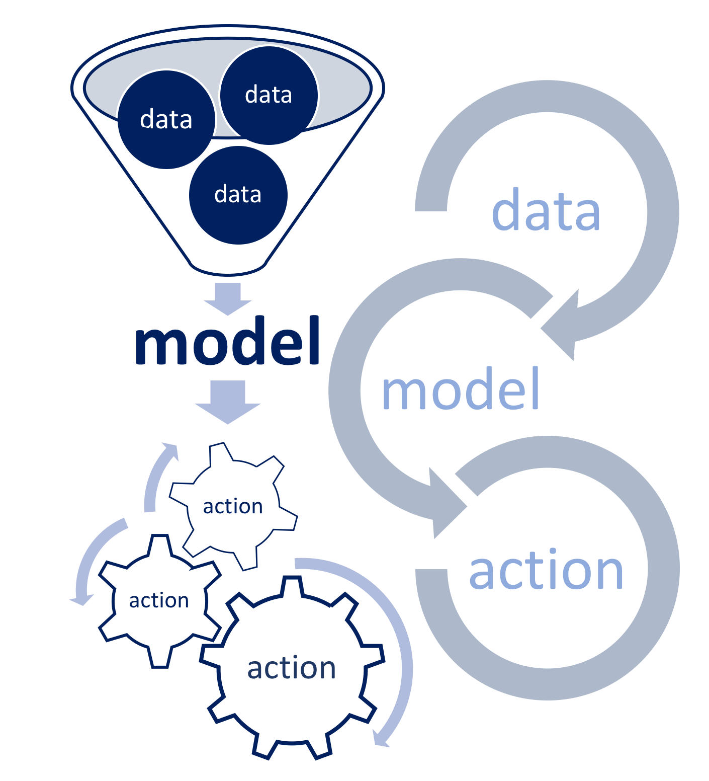
This section introduces you to fundamental Machine Learning (ML) concepts and algorithms. Empowered by modern computing capabilities and statistical modelling, machine scale analysis can capture hidden values in big data that are otherwise limited to human scale thinking. In 1959, in a paper Some Studies in Machine Learning Using the Game of Checkers Arthur Samuel used the term machine learning in the game of checkers in the form we know it today: “to verify the fact that a computer can be programmed so that it will learn to play a better game of checkers than can be played by the person who wrote the program”. The paper conveys the process of passing our own methods of learning to a machine as a subfield of statistical computing. It is the application of statistical modelling to obtain a general understanding of the data, to make predictions and to improve performance based on data and empirical information.

ML can learn from the data that is processed and analysed and the more data it processes, the more it can learn. But, to create such intelligent machines it is useful to develop an understanding of classical statistics that is the LifeBlood of ML algorithms. Coated by the layers of k-nearest neighbours, linear regression, random forest, naïve bayes… machines can develop the cognitive abilities of today’s Artificial Intelligence (AI).

Translating the statistical methodologies that can run on machines through coding and programming is another vital part of ML. As such, R is a powerful statistical language for learning an important and desirable ML skill: code writing for statistical modelling. Using R greatly simplifies machine learning. Using R enables us to focus on developing an understanding of how each algorithm can solve a problem, for which we can simply use a written package to quickly generate prediction models on data with a few command lines.

Types of ML

We will touch upon a few of the most popular ML algorithms from a vast set of its algorithmic tools for understanding data. These tools are broadly classified as supervised or unsupervised. In general, supervised learning involves building a statistical model for estimating or predicting an output based on one or more inputs. There are many examples of their application in pharma and medicine, such as disease identification/diagnosis and personalised treatments, or pricing in business to name a few. With unsupervised learning, there are inputs but no supervising output; nevertheless, we can learn relationships and structure from such data. One of the most popular examples is a recommender system as a reflection of our consumer behaviour. Other examples can be found in biological genomic studies, market research, security, with the most used example being anomaly detection of malicious activity in an organization’s network etc.

Fuelled by powered computer technologies ML models have evolved considerably in the last decade, advancing into a third category known as reinforcement. Unlike supervised and unsupervised learning, reinforcement learning continuously improves its model advancing from the previous iterations. This differs from the other two categories of ML, which reach an indefinite stage after the model is formulated from the training and test data segments. Examples can be found in computer gaming, skill acquisition such as real time discussion etc.

Supervised Versus Unsupervised Learning

The majority of data analysis problems fall into one of the two ML categories: supervised or unsupervised. Sometimes we deal with a problem in which for each observation we have a predictor(s) \(x_i\), \(i = 1, 2, … n\) there is a response \(y_i\). In those cases, we seek to find a model that reflects the possible relationship between response and predictor(s). The aim is to be able to predict the response values for future observation accurately, with greater understanding of the relationship between the two. In statistical terms, we wish to conduct:

• the prediction of \(y\)’s for future values of \(x\)’s and
• the inference about the nature of the relationship between \(X\) and \(Y\)

The best known statistical modelling techniques that fall into this ML category that are commonly used are linear regression, logistic regression, Generalised Additive Models (GAM), boosting and Support Vector Machines (SVM).

To the problems where for each observation \(i = 1, 2, … n\) we have a set of measurements \(x_i\), but no associated responses \(y_i\) based on which we can “supervise” the analysis to understand the relationship between the variables or between the observations, we referred to as unsupervised learning. Commonly used methodology in this setting is clustering. The goal of cluster analysis is to group the observation in the data set into disjointed clusters of similar samples. It is commonly used in market segmentation where, for example, you need to develop marketing strategies for identified groups of customers clustered into them based on their behaviour.

Previously, we recognised that when dealing with the measured response variable in statistical modelling we tended to use regression. If, however we have attribute response variables such as defaults on a debt, gender, ethnicity, to name a few, we tend to use classification modelling. In multifactor data analysis, selecting the appropriate statistical modelling technique is not so straightforward as it is in bivariate statistical modelling situations, for which we fit a model based on the type of response variable. Here, we can use logistic regression for the models with binary response attribute variables as it estimates class probabilities, which on the other hand can be thought of as a regression method as well. Methods such as K-nearest neighbours and boosting can be used for both measured and attribute response variables. When dealing with multifactor statistical modelling, we have to think carefully not just about the type of response variable, but most of all about the type of problems we wish to address.

Assessing Model Accuracy

Selecting the most efficient approach can be one of the most challenging parts of performing statistical modelling in practice, as the choice of the model that has worked on one data set may not perform as well on another similar data set. Therefore, evaluating the performance of a chosen statistical method is seen as an important part of statistical modelling.

Through statistical modelling, we are trying to explain and dig deeper into understanding the nature of a process, i.e. phenomena of interest. We describe this phenomenon as an unknown function \(f\). In its related data we annotate as \(x\) the information that can explain the problem’s behaviour (this could be a single value or a vector or matrix of values or something more complex) and as \(y\) the results of its behaviour (this could also be a single value or something more complex). Mathematically we present this as

\[y_i = f(x_i)\]

However, there is one more element we need to add to this equation that would make it statistically correct

\[y_i = f(x_i) + \epsilon_i\]

We refer to this additional element epsilon as an “error” and it depicts the noise, the variation of the \(f\)’s behaviour. The standard approach is to adopt the following distribution structure: \(\epsilon \sim N(0,\sigma)\), meaning that the \(\epsilon\) value is considered to be normally distributed with a mean of \(0\) and some standard deviation \(\sigma\). This implies that negative and positive impacts from this noise are considered equally likely, and that small errors are much more likely than extreme ones.

To evaluate the performance of a statistical model on a given data set, we commonly monitor the discrepancies between the predicted response values for given observations obtained by the chosen statistical model (\(\hat{f}(x_i)\)) and the true response values for these observations (\(y_i\)). The most commonly used measure is the mean squared error (MSE):

\[MSE = \frac{1}{n} \sum^{n}_{i=1}(y_i - \hat{f}(x_i))^2\]

It is easy to note that the small \(MSE\) will correspond to the model for which the predicted responses (\(\hat{f}(x_i)\)) are very close to the true responses (\(y_i\)) and large if the true and predicted responses differ significantly.

In general, a machine learning model aims to make good predictions on new, previously unseen data. However, we don’t have the previously unseen data when experimenting with a new problem. One way of overcoming this obstacle is to split the given data into two subsets:

• training data: a subset to train a model
• test data: a subset to test the model

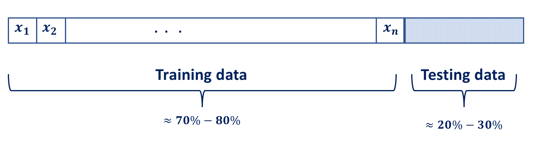
The ratio of of two split should be approximately 75/25. This means that training data should account for around 75 percent of the rows in the given data and the other 25 percent of rows is the test data. Good performance on the test data is a useful indicator of good performance on the new data in general, assuming that the test data is sufficiently large and that you don’t take advantage of using the same test data over and over again to make your model look better than it is. Often data is arranged sequentially and it is good practice to randomise the rows in the data set prior to the split, as it helps to avoid bias in the fitted model. The easiest way to split the data into a training and test set is to take a random sample.

But we have already discussed that we are not really interested how well the model “works training” on the training data, ie. \(\hat{f}(x_i) \approx y_i\). We are more interested in the accuracy of the predictions \(\hat{f}(x_0)\) that are obtained when we apply the model to previously unseen test data \((x_0, y_0)\), ie. \(\hat{f}(x_0) \approx y_0\). In other words, we want to chose the model with the lowest \(test\) \(MSE\) and to do so we need a large enough number of observations in the test data to calculate the mean square prediction error for the test observations (\(x_0\), \(y_0\)), to which we can refer to as the \(test\) \(MSE\).

\[mean(y_0 - \hat{f}(x_0))^2\]

In statistics nothing is black and white. In other words, nothing is straightforward and there are many considerations one needs to take into account when applying statistical modelling. The same applies in this situation. We need to realise that when a given model yields a small training MSE but a large test MSE, we are said to be overfitting the data. The statistical model is too ‘preoccupied’ to find patterns in the training data and consequently is modelling the patterns that are caused by random effect, rather than by true features of the unknown function \(f\). When the model overfits the training data, the test MSE will be large because the modelled features that the model identifies in the training data just do not exist in the test data. Saying that, regardless of overfitting occurring or not, we expect the training MSE to be smaller than the test MSE, as most of the statistical models either directly or indirectly seek to minimize the training MSE. We need to be aware that the chosen model needs to be flexible and not rigid and glued to the training data.

Reducible and Irreducible Error: The Bias-Variance Trade-Off

MSE is simple to calculate and yet, despite its simplicity, it can provide us with a vital insight into modelling. It consists of two intrinsic components:

• bias
• variance

that can provide greater enlightenment about how the model works.

We have talked earlier about variance in general, but we have not explained the idea of bias in statistical term. Bias is the average difference between the estimator \(\hat{y}\) and true value \(y\). Mathematically we write bias as:

\[E[\hat{y} – y]\]

As it is not squared difference, it can be either positive or negative. Positive or negative bias implies that the model is over or under “predicting”, while the value of zero would indicate that the model is likely to predict too much as it is to predict too little. The latter implies that the model can be completely wrong in its prediction and still provide us with the bias of zero. This implies that bias on its own provides little information about how correct the model is in its prediction.

Remember that \(y = f(x) + \epsilon\) and therefore \(\hat{f}\) is not directly approximating \(f\). \(\hat{f}\) models \(y\) that includes the noise. It can be challenging and in some cases even impossible to meaningfully capture the behaviour of \(f\) itself when the noise term is very large. We have discussed earlier that we assess model accuracy using MSE which is calculated by

1. obtaining the error (i.e. discrepancy between \(\hat{f}(x_i)\) and \(y_i\))
2. squaring this value (making negative into the positive same, and greater error gets more severe penalty)
3. then averaging these results

The mean of the squared error is the same as the expectation\(^*\) of our squared error so we can go ahead and simplify this a slightly:

\[MSE=E[(y-\hat{f}(x))^2]\] Now, we can break this further and write it as \[MSE = E[(f(x)+ \epsilon - \hat{f}(x))^2]\] Knowing that computing the expectation of adding two random variables is the same as computing the expectation of each random variable and then adding them up

\[E[X+Y]=E[X] +E[Y]\] and recalling that \(\sigma^2\) represent the variance of \(\epsilon\), where the variance is calculated as \[E[X^2]-E[X]^2,\] and therefore \[Var(\epsilon) = \sigma^2 = E[\epsilon^2] - E[\epsilon]^2,\] with \(\epsilon \sim N(0,\sigma)\)

\[E[\epsilon]^2=\mu^2=0^2=0\] we get

\[E[\epsilon^2] = \sigma^2\] This helps us to rearranging MSE further and calculate it as

\[MSE=σ^2+E[−2f(x)\hat{f}(x)+f(x)^2+\hat{f}(x)^2],\]

where \(\sigma^2\) is the variance of the noise, ie. \(\epsilon\). This is a “eureka” moment: the variance of the noise in data is an irreducible part of the MSE. Regardless of how good the model is, it can never reduce the MSE to being less than the variance related to the noise, i.e. error. This error represents the lack of information in data used to adequately explain everything that can be known about the phenomena being modelled. We should not look at it as a nuisance, as it can often guide us to further explore the problem and look into other factors that might be related to it.

Knowing that \[Var(X) = E[X^2] - E[X]^2,\] we can apply further transformation and break MSE into \[MSE = \sigma^{2}+Var[f(x)-\hat{f}(x)]+E[f(x)-\hat{f}(x)]^2\] The term \(Var[f(x)-\hat{f}(x)]\) is the variance in the model predictions from the true output values and the last term \(E[f(x)-\hat{f}(x)]^2\) is just the bias squared. We mentioned earlier that that unlike variance, bias can be positive or negative, so we square this value in order to make sure it is always positive.

With this in mind, we realise that MSE consists of:

1. model variance
2. model bias and
3. irreducible error

\[\text{Mean Squared Error}=\text{Model Variance} + \text{Model Bias}^2 + \text{Irreducible Error}\]

We come to the conclusion that in order to minimize the expected test error, we need to select a statistical model that simultaneously achieves low variance and low bias.

💡 Note that in practice we will never know what the variance \(\sigma^2\) of the error \(\epsilon\) is, and therefore we will not be able to determine the variance and the bias of the model. However, since \(\sigma^2\) is constant, to improve the model we have to decrease either bias or variance.

Testing the model using the test data and observing its bias and variance can help us address some important issues, allowing us to reason with the model. If the model fails to find the \(f\) in data and is systematically over or under predicting, this will indicate underfitting and it will be reflected through high bias. However, high variance when working with test data indicates the issue of overfitting. What happens is that the model has learnt the training data really well and is too close to the data, so much so that it starts to mistake the \(f(x) + \epsilon\) for true \(f(x)\).

Simulation Study

To understand these concepts, let us run a small simulation study. We will:

1. simulate a function \(f\)
2. apply the error, i.e. noise sampled from a distribution with a known variance

To make it very simple and illustrative we will use a linear function \(f(x) = 3 + 2x\) to simulate response \(y\) with the error \(e\thicksim N(\mu =0, \sigma^2 =4)\), where \(x\) is going to be a sequence of numbers between \(0\) and \(10\) in steps of \(0.1\). We will examine the simulations for the models that over and under estimate the true \(f\), and since it is a linear function we will not have a problem identifying using simple linear regression modelling.

Let’s start with a simulation in which we will model the true function with \(\hat{f}_{1} = 4 + 2x\) and \(\hat{f}_{2} = 1 + 2x\).

set.seed(123) ## set the seed of R‘s random number generator

# simulate function f(x) = 3 + 2x
f <- function(x){
  3 + 2 * x 
}
# generate vector X
x <- seq(0, 10, by = 0.05)
# the error term coming from N(mean = 0, variance = 4)
e <- rnorm(length(x), mean = 0, sd = 2)
# simulate the response vector Y
y <- f(x) + e

# plot the simulated data 
plot(x, y, cex = 0.75, pch = 16, main = "Simulation: 1") 
abline(3, 2, col ="gray", lwd = 2, lty = 1)
# model fitted to simulated data
f_hat_1<- function(x){
  4 + 2 * x
}
f_hat_2 <- function(x){
  1 + 2 * x
}
y_bar = mean(y) # average value of the response variable y
f_hat_3 <- function(x){
  y_bar
}
# add the line representing the fitted model
abline(1, 2, col = "red", lwd = 2, lty = 2)
abline(4, 2, col = "blue", lwd = 2, lty = 1)
abline(y_bar, 0, col = "darkgreen", lwd = 2, lty = 3)
legend(7.5, 10, legend=c("f_hat_1", "f_hat_2", "f_hat_3", "f"),
       col = c("blue", "red", "darkgreen", "gray"), 
       lwd = c(2, 2, 2, 2), lty = c(1:3, 1),
       text.font = 4, bg = 'lightyellow')

Observing the graph, we notice that \(\hat{f}_1\) and \(\hat{f}_2\), depicted in blue and red lines respectively, follow the data nicely, but are also systematically over (in the case of \(\hat{f}_1\) and under (in the case of \(\hat{f}_2\)) estimating the values. In the simple model \(\hat{f}_3\), the line represents the value \(\bar{y}\), which cuts the data in half.

As we mentioned earlier, knowing the true function \(f\) and the distribution of \(\epsilon\) we can calculate: - the MSE using the simulated data and the estimated model, - the model’s bias and variance which will allow for the calculation of the “theoretical” MSE. This will allow for more detailed illustration about the information contained in the model’s bias and variance.

# calculate MSE from data
MSE_data1 = mean((y - f_hat_1(x))^2)
MSE_data2 = mean((y - f_hat_2(x))^2)
MSE_data3 = mean((y - f_hat_3(x))^2)
# model bias 
bias_1 = mean(f_hat_1(x) - f(x))
bias_2 = mean(f_hat_2(x) - f(x))
bias_3 = mean(f_hat_3(x) - f(x))
# model variance
var_1 = var(f(x) - f_hat_1(x))
var_2 = var(f(x) - f_hat_2(x))
var_3 = var(f(x) - f_hat_3(x))
# calculate 'theoretical' MSE
MSE_1 = bias_1^2 + var_1 + 2^2
MSE_2 = bias_2^2 + var_2 + 2^2
MSE_3 = bias_3^2 + var_3 + 2^2
for (i in 1:1){
  cat (c("==============================================","\n"))
  cat (c("=============== f_hat_1 ================","\n"))
  cat(c("MSE_data1 = ", round(MSE_data1, 2),  sep = '\n'))
  cat(c("bias_1 = ", bias_1, sep = '\n' ))   
  cat(c("variance_1 = ", round(var_1, 2), sep = '\n' ))  
  cat(c("MSE_1 = 4 + bias_1^2 + variance_1 = ", MSE_1, sep = '\n' )) 
  cat(c("==============================================","\n"))
  cat(c("=============== f_hat_2 ================","\n"))
  cat(c("MSE_data2 = ", round(MSE_data2, 2),  sep = '\n'))
  cat(c("bias_2 = ", bias_2, sep = '\n' ))   
  cat(c("variance_2 = ", round(var_2, 2), sep = '\n' ))  
  cat(c("MSE_2 = 4 + bias_2^2 + variance_2 = ", MSE_2, sep = '\n' ))
  cat(c("==============================================","\n"))
  cat(c("=============== f_hat_3 ================","\n"))
  cat(c("average y = ", round(y_bar, 2),  sep = '\n'))
  cat(c("MSE_data3 = ", round(MSE_data3, 2),  sep = '\n'))
  cat(c("bias_3 = ", round(bias_3, 2), sep = '\n' ))   
  cat(c("variance_3 = ", round(var_3, 2), sep = '\n' ))  
  cat(c("MSE_3 = 4 + bias_3^2 + variance_3 = ", round(MSE_3, 2), sep = '\n' ))
  cat(c("==============================================","\n"))
}

## ============================================== 
## =============== f_hat_1 ================ 
## MSE_data1 =  4.61 
## bias_1 =  1 
## variance_1 =  0 
## MSE_1 = 4 + bias_1^2 + variance_1 =  5 
## ============================================== 
## =============== f_hat_2 ================ 
## MSE_data2 =  7.64 
## bias_2 =  -2 
## variance_2 =  0 
## MSE_2 = 4 + bias_2^2 + variance_2 =  8 
## ============================================== 
## =============== f_hat_3 ================ 
## average y =  13 
## MSE_data3 =  36.7 
## bias_3 =  0 
## variance_3 =  33.84 
## MSE_3 = 4 + bias_3^2 + variance_3 =  37.84 
## ==============================================

\(\hat{f}_1\) has a positive bias because it is overestimating data points more often than it is underestimating, but as it does it so consistently in comparison to \(f\) that produces variance of zero. In contrast \(\hat{f}_2\) has a negative bias as it is underestimating simulated data, but nonetheless it also does it consistently, resulting in zero variance with \(f\).

Unlike in the previous two model estimates which follow the data points, \(\hat{f}_3\) predicts the mean value of data, resulting in no bias since it evenly underestimates and overestimates \(f(x)\). However, the variation in prediction between \(f\) and \(\hat{f}_3\) is obvious.

Given that the true function \(f\) is linear, by applying simple regression modelling, we should be able to estimate it easily in R using the \(lm()\) function.

# model fitted to simulated data
f_hat_4<- function(x){
    lm(y~x)
}
# plot the simulated data 
plot(x, y, cex = 0.75, pch = 16, main = "Simulation: 2") 
abline(3, 2, col ="gray", lwd = 2, lty = 1)
# add the line representing the fitted model
abline(lm(y~x), col ="red", lwd = 2, lty = 3)
legend(7.5, 8, legend=c("f_hat_4", "f"),
       col = c("red", "gray"), 
       lwd = c(2, 2), lty = c(3, 1),
       text.font = 4, bg = 'lightyellow')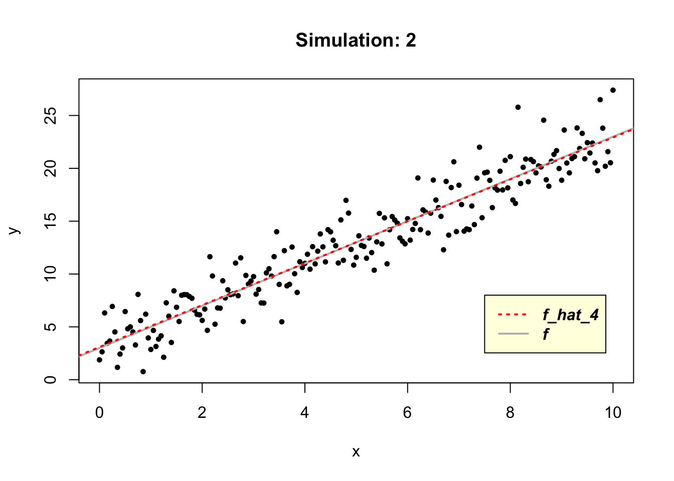

Since the true function \(f\) is a linear model it is not surprising that \(\hat{f}_4\) can learn it, resulting in zero values of the model’s bias and variance.

# calculate MSE from data
MSE_data4 = mean((y - predict(f_hat_4(x)))^2)
# model bias 
bias_4 = mean(predict(f_hat_4(x)) - f(x))
# model variance
var_4 = var(f(x) - predict(f_hat_4(x)))
# calculate 'theoretical' MSE
MSE_4 = bias_4^2 + var_4 + 2^2
for (i in 1:1){
  
  cat (c("==============================================","\n"))
  cat (c("=============== f_hat_4 ================","\n"))
  cat(c("MSE_data4 = ", round(MSE_data4, 2),  sep = '\n'))
  cat(c("bias_4 = ", round(bias_4, 2), sep = '\n' ))   
  cat(c("variance_4 = ", round(var_4, 2), sep = '\n' ))  
  cat(c("MSE_4 = 4 + bias_4^2 + variance_4 = ", round(MSE_4, 2), sep = '\n' ))
  cat (c("==============================================","\n"))
}

## ============================================== 
## =============== f_hat_4 ================ 
## MSE_data4 =  3.62 
## bias_4 =  0 
## variance_4 =  0 
## MSE_4 = 4 + bias_4^2 + variance_4 =  4 
## ==============================================

We realise that the \(MSE\) is more than just a simple error measurement. It is a tool that informs and educates the modeller about the performance of the model being used in the analysis of a problem. It is packed with information that when unwrapped can provide a greater insight into not just the fitted model, but the nature of the problem and its data. It provides you with the desired agility for steering a boat in a sea of data.

\(^*\) The Expectation of a Random Variable is the sum of its values weighted by their probability. For example: What is the average toss of a fair six-sided die?

If the random variable is the top face of a tossed, fair six-sided die, then the probability of die landing on \(X\) is

\[f(x) = \frac{1}{6}\] for \(x = 1, 2,... 6\). Therefore, the average toss, i.e. the expected value of \(X\) is:

\[E(X) = 1(\frac{1}{6}) + 2(\frac{1}{6}) + 3(\frac{1}{6}) + 4(\frac{1}{6}) + 5(\frac{1}{6}) + 6(\frac{1}{6}) = 3.5\] Of course, we do not expect to get a fraction when tossing a die, i.e. we do not expect the toss to be 3.5, but rather an integer number between 1 to 6. So, what the expected value is really saying is what is the expected average of a large number of tosses will be. If we toss a fair, six-side die hundreds of times and calculate the average of the tosses we will not get the exact 3.5 figure, but we will expect it to be close to 3.5. This is a theoretical average, not the exact one that is realised.

YOUR TURN 👇

1. Identify a data set from your own work experience or from amongst many available freely on the Internet and describe a problem that can be addressed using this data. Write a brief report describing the identified data and a problem that can be addressed using this data. Discuss further in your report which of the categories of ML would be applicable for the analysis of this problem? Try to justify your thinking.

2. In the simulation study, notice the difference between \(MSE\) calculated from the simulated data and the one we obtain by plugging in the values of \(\sigma^2\) and estimator’s \(bias\) and \(variance\). Try to increase the sample size of the simulation and comment on the changes you may notice (hint: make a change for smaller steps in the \(seq()\) function). Can you draw any conclusions; what are they?

© 2020 Tatjana Kecojevic