Subset Variable Selection
This short tutorial on Subset variable Selection in R comes from pp. 244-251 of “Introduction to Statistical Learning with Applications in R” by Gareth James, Daniela Witten, Trevor Hastie and Robert Tibshirani and chapter “Forward, Backward, and Stepwise Selection”, from pp. 511-519 of “Applied Predictive Modeling” by Max Kuhn.
For the large numbers of explanatory variables, and many interactions and non-linear terms, the process of model simplification can take a very long time. There are many algorithms for automatic variable selection that can help to chose the variables to include in a regression model.
Using Best Subsets Regression and Stepwise Regression
Stepwise regression and Best Subsets regression (BREG) are two of the more common variable selection methods. The stepwise procedure starts from the saturated model (or the maximal model, whichever is appropriate) through a series of simplifications to the minimal adequate model. This progression is made on the basis of deletion tests: F tests, AIC, t-tests or chi-squared tests that assess the significance of the increase in deviance that results when a given term is removed from the current model.
The BREG, also known as “all possible regressions”, as the name of the procedure indicates, fits a separate least squares regression for each possible combination of the \(p\) predictors, i.e. explanatory variables. After fitting all of the models, BREG then displays the best fitted models with one explanatory variable, two explanatory variables, three explanatory variables, and so on. Usually, either adjusted R-squared or Mallows Cp is the criterion for picking the best fitting models for this process. The result is a display of the best fitted models of different sizes up to the full/maximal model and the final fitted model can be selected by comparing displayed models based on the criteria of parsimony.
Case Study
We want to apply the subset selection approach to the fat data, available in the library(faraway).
We wish to predict body fat (variable brozek) using all predictors except for siri, density and free.
As instructed, we will start off by creating a subset of all the variables from the fat data set except for siri, density and free. We will save this subset as a new data frame bodyfat. To confirm that the three suggested variables have been removed, we will check for the difference in the dimension of the two data frames and have a glimpse at teh data.
#If you don't have the "ISLR" package installed yet, uncomment and run the line below
#install.packages("ISLR")
library(ISLR)
library(faraway)
library(tidyr)
suppressPackageStartupMessages(library(dplyr))
bodyfat <- fat %>%
  select(-siri, -density, -free)
dim(fat) - dim(bodyfat)
## [1] 0 3glimpse(bodyfat)## Rows: 252
## Columns: 15
## $ brozek <dbl> 12.6, 6.9, 24.6, 10.9, 27.8, 20.6, 19.0, 12.8, 5.1, 12.0, 7.5,…
## $ age <int> 23, 22, 22, 26, 24, 24, 26, 25, 25, 23, 26, 27, 32, 30, 35, 35…
## $ weight <dbl> 154.25, 173.25, 154.00, 184.75, 184.25, 210.25, 181.00, 176.00…
## $ height <dbl> 67.75, 72.25, 66.25, 72.25, 71.25, 74.75, 69.75, 72.50, 74.00,…
## $ adipos <dbl> 23.7, 23.4, 24.7, 24.9, 25.6, 26.5, 26.2, 23.6, 24.6, 25.8, 23…
## $ neck <dbl> 36.2, 38.5, 34.0, 37.4, 34.4, 39.0, 36.4, 37.8, 38.1, 42.1, 38…
## $ chest <dbl> 93.1, 93.6, 95.8, 101.8, 97.3, 104.5, 105.1, 99.6, 100.9, 99.6…
## $ abdom <dbl> 85.2, 83.0, 87.9, 86.4, 100.0, 94.4, 90.7, 88.5, 82.5, 88.6, 8…
## $ hip <dbl> 94.5, 98.7, 99.2, 101.2, 101.9, 107.8, 100.3, 97.1, 99.9, 104.…
## $ thigh <dbl> 59.0, 58.7, 59.6, 60.1, 63.2, 66.0, 58.4, 60.0, 62.9, 63.1, 59…
## $ knee <dbl> 37.3, 37.3, 38.9, 37.3, 42.2, 42.0, 38.3, 39.4, 38.3, 41.7, 39…
## $ ankle <dbl> 21.9, 23.4, 24.0, 22.8, 24.0, 25.6, 22.9, 23.2, 23.8, 25.0, 25…
## $ biceps <dbl> 32.0, 30.5, 28.8, 32.4, 32.2, 35.7, 31.9, 30.5, 35.9, 35.6, 32…
## $ forearm <dbl> 27.4, 28.9, 25.2, 29.4, 27.7, 30.6, 27.8, 29.0, 31.1, 30.0, 29…
## $ wrist <dbl> 17.1, 18.2, 16.6, 18.2, 17.7, 18.8, 17.7, 18.8, 18.2, 19.2, 18…Using the glimpse() function allows us to notice that all the variables in our new bodyfat data set are the measured type.
Get to Know Your Data
Let us take a look at the data using the DT package, which provides an R interface to the JavaScript library DataTables. It will enable us to filter through the displayed data and quickly check for NAs to see if there are any missing values that should be of concern.
DT::datatable(fat)Alternatively, we can use the is.na() function to check if there are any missing observations in particular with respect to the response variable bronzek. For a given input vector the is.na() function returns a vector of TRUE and FALSE value, with a value of TRUE for any elements that are missing, and a FALSE value for non-missing elements. By using the sum() function we can then count all of the missing elements, which can be easily removed from data by using either the na.omit() function or the drop_na function.
bodyfat %>%
  select(brozek) %>%
  is.na() %>%
  sum()
## [1] 0The correlation matrix and its visualisation
Previously (see the section on Multiple Regression), we learnt how to examine multivariate data by creating a scatter plot matrix to obtain an in-depth vision into its behaviour. We used the GGally::ggpairs() function that produces a pairwise comparison of multivariate data for both data types: measured and attribute. Creating such a matrix for a data set with a considerable number of variables could be a taxing task with a resulting display that may not be easy to make sense of.
Fabulous Frank Harrell (check his blog Statistical Thinking if you haven’t stumbled upon it yet!) has created the Hmisc package with many useful functions for data analysis and high-level graphics. It contains the rcorr function for the computation of Pearson or Spearman correlation matrix with pairwise deletion of missing data. It generates one table of correlation coefficients, i.e. the correlation matrix and another table of the \(p\)-values.
bodyfat.rcorr = Hmisc::rcorr(as.matrix(bodyfat))
bodyfat.coeff = bodyfat.rcorr$r
bodyfat.p = bodyfat.rcorr$P
bodyfat.coeff
## brozek age weight height adipos neck
## brozek 1.00000000 0.28917352 0.61315611 -0.08910641 0.72799418 0.4914889
## age 0.28917352 1.00000000 -0.01274609 -0.17164514 0.11885126 0.1135052
## weight 0.61315611 -0.01274609 1.00000000 0.30827854 0.88735216 0.8307162
## height -0.08910641 -0.17164514 0.30827854 1.00000000 -0.02489094 0.2537099
## adipos 0.72799418 0.11885126 0.88735216 -0.02489094 1.00000000 0.7778569
## neck 0.49148893 0.11350519 0.83071622 0.25370988 0.77785691 1.0000000
## chest 0.70288516 0.17644968 0.89419052 0.13489181 0.91179865 0.7848350
## abdom 0.81370622 0.23040942 0.88799494 0.08781291 0.92388010 0.7540774
## hip 0.62569993 -0.05033212 0.94088412 0.17039426 0.88326922 0.7349579
## thigh 0.56128438 -0.20009576 0.86869354 0.14843561 0.81270609 0.6956973
## knee 0.50778587 0.01751569 0.85316739 0.28605321 0.71365983 0.6724050
## ankle 0.26678256 -0.10505810 0.61368542 0.26474369 0.50031664 0.4778924
## biceps 0.49303089 -0.04116212 0.80041593 0.20781557 0.74638418 0.7311459
## forearm 0.36327744 -0.08505555 0.63030143 0.22864922 0.55859425 0.6236603
## wrist 0.34757276 0.21353062 0.72977489 0.32206533 0.62590659 0.7448264
## chest abdom hip thigh knee ankle
## brozek 0.7028852 0.81370622 0.62569993 0.5612844 0.50778587 0.2667826
## age 0.1764497 0.23040942 -0.05033212 -0.2000958 0.01751569 -0.1050581
## weight 0.8941905 0.88799494 0.94088412 0.8686935 0.85316739 0.6136854
## height 0.1348918 0.08781291 0.17039426 0.1484356 0.28605321 0.2647437
## adipos 0.9117986 0.92388010 0.88326922 0.8127061 0.71365983 0.5003166
## neck 0.7848350 0.75407737 0.73495788 0.6956973 0.67240498 0.4778924
## chest 1.0000000 0.91582767 0.82941992 0.7298586 0.71949640 0.4829879
## abdom 0.9158277 1.00000000 0.87406618 0.7666239 0.73717888 0.4532227
## hip 0.8294199 0.87406618 1.00000000 0.8964098 0.82347262 0.5583868
## thigh 0.7298586 0.76662393 0.89640979 1.0000000 0.79917030 0.5397971
## knee 0.7194964 0.73717888 0.82347262 0.7991703 1.00000000 0.6116082
## ankle 0.4829879 0.45322269 0.55838682 0.5397971 0.61160820 1.0000000
## biceps 0.7279075 0.68498272 0.73927252 0.7614774 0.67870883 0.4848545
## forearm 0.5801727 0.50331609 0.54501412 0.5668422 0.55589819 0.4190500
## wrist 0.6601623 0.61983243 0.63008954 0.5586848 0.66450729 0.5661946
## biceps forearm wrist
## brozek 0.49303089 0.36327744 0.3475728
## age -0.04116212 -0.08505555 0.2135306
## weight 0.80041593 0.63030143 0.7297749
## height 0.20781557 0.22864922 0.3220653
## adipos 0.74638418 0.55859425 0.6259066
## neck 0.73114592 0.62366027 0.7448264
## chest 0.72790748 0.58017273 0.6601623
## abdom 0.68498272 0.50331609 0.6198324
## hip 0.73927252 0.54501412 0.6300895
## thigh 0.76147745 0.56684218 0.5586848
## knee 0.67870883 0.55589819 0.6645073
## ankle 0.48485454 0.41904999 0.5661946
## biceps 1.00000000 0.67825513 0.6321264
## forearm 0.67825513 1.00000000 0.5855883
## wrist 0.63212642 0.58558825 1.0000000bodyfat.p## brozek age weight height adipos
## brozek NA 3.044832e-06 0.000000e+00 1.584527e-01 0.00000000
## age 3.044832e-06 NA 8.404326e-01 6.303967e-03 0.05956386
## weight 0.000000e+00 8.404326e-01 NA 5.989982e-07 0.00000000
## height 1.584527e-01 6.303967e-03 5.989982e-07 NA 0.69415116
## adipos 0.000000e+00 5.956386e-02 0.000000e+00 6.941512e-01 NA
## neck 0.000000e+00 7.206646e-02 0.000000e+00 4.614130e-05 0.00000000
## chest 0.000000e+00 4.966465e-03 0.000000e+00 3.231539e-02 0.00000000
## abdom 0.000000e+00 2.249495e-04 0.000000e+00 1.646071e-01 0.00000000
## hip 0.000000e+00 4.263055e-01 0.000000e+00 6.701323e-03 0.00000000
## thigh 0.000000e+00 1.408117e-03 0.000000e+00 1.838840e-02 0.00000000
## knee 0.000000e+00 7.820168e-01 0.000000e+00 3.927576e-06 0.00000000
## ankle 1.770467e-05 9.609999e-02 0.000000e+00 2.062620e-05 0.00000000
## biceps 0.000000e+00 5.153980e-01 0.000000e+00 9.038055e-04 0.00000000
## forearm 2.808188e-09 1.783211e-01 0.000000e+00 2.519644e-04 0.00000000
## wrist 1.446366e-08 6.442181e-04 0.000000e+00 1.721428e-07 0.00000000
## neck chest abdom hip thigh
## brozek 0.000000e+00 0.000000e+00 0.000000e+00 0.000000000 0.000000000
## age 7.206646e-02 4.966465e-03 2.249495e-04 0.426305473 0.001408117
## weight 0.000000e+00 0.000000e+00 0.000000e+00 0.000000000 0.000000000
## height 4.614130e-05 3.231539e-02 1.646071e-01 0.006701323 0.018388401
## adipos 0.000000e+00 0.000000e+00 0.000000e+00 0.000000000 0.000000000
## neck NA 0.000000e+00 0.000000e+00 0.000000000 0.000000000
## chest 0.000000e+00 NA 0.000000e+00 0.000000000 0.000000000
## abdom 0.000000e+00 0.000000e+00 NA 0.000000000 0.000000000
## hip 0.000000e+00 0.000000e+00 0.000000e+00 NA 0.000000000
## thigh 0.000000e+00 0.000000e+00 0.000000e+00 0.000000000 NA
## knee 0.000000e+00 0.000000e+00 0.000000e+00 0.000000000 0.000000000
## ankle 8.881784e-16 4.440892e-16 3.597123e-14 0.000000000 0.000000000
## biceps 0.000000e+00 0.000000e+00 0.000000e+00 0.000000000 0.000000000
## forearm 0.000000e+00 0.000000e+00 0.000000e+00 0.000000000 0.000000000
## wrist 0.000000e+00 0.000000e+00 0.000000e+00 0.000000000 0.000000000
## knee ankle biceps forearm wrist
## brozek 0.000000e+00 1.770467e-05 0.000000e+00 2.808188e-09 1.446366e-08
## age 7.820168e-01 9.609999e-02 5.153980e-01 1.783211e-01 6.442181e-04
## weight 0.000000e+00 0.000000e+00 0.000000e+00 0.000000e+00 0.000000e+00
## height 3.927576e-06 2.062620e-05 9.038055e-04 2.519644e-04 1.721428e-07
## adipos 0.000000e+00 0.000000e+00 0.000000e+00 0.000000e+00 0.000000e+00
## neck 0.000000e+00 8.881784e-16 0.000000e+00 0.000000e+00 0.000000e+00
## chest 0.000000e+00 4.440892e-16 0.000000e+00 0.000000e+00 0.000000e+00
## abdom 0.000000e+00 3.597123e-14 0.000000e+00 0.000000e+00 0.000000e+00
## hip 0.000000e+00 0.000000e+00 0.000000e+00 0.000000e+00 0.000000e+00
## thigh 0.000000e+00 0.000000e+00 0.000000e+00 0.000000e+00 0.000000e+00
## knee NA 0.000000e+00 0.000000e+00 0.000000e+00 0.000000e+00
## ankle 0.000000e+00 NA 4.440892e-16 3.886669e-12 0.000000e+00
## biceps 0.000000e+00 4.440892e-16 NA 0.000000e+00 0.000000e+00
## forearm 0.000000e+00 3.886669e-12 0.000000e+00 NA 0.000000e+00
## wrist 0.000000e+00 0.000000e+00 0.000000e+00 0.000000e+00 NALooking at the figures above, we notice that the response variable brozek is in strong association with all of the explanatory variables from the data set. In fact, it looks as if all variables are in strong correlation with one another, with a very few exceptions such as in the case of height and adipos, hip and age, weight and age to name a few of the most obvious ones. In an example like this one, where there are a high number of variables to consider, it is useful to visualise the correlation matrix. There are several packages available for the visualisation of a correlation matrix in R:
GGally- extension toggplot2ggpairs()function
ggcorrplot- visualisation of a correlation matrix usingggplot2ggcorrplot()function
corrplot- rich visualisation of a correlation matrixcorrplot.mixed()function
corrr- a tool for exploring correlationsnetwork_plot()function
corrgram- calculates correlation of variables and displays the results graphically, based on the Corrgrams: Exploratory displays for correlation matrices paper (Friendly, 2002)corrgramfunction
PerformanceAnalytics- package of econometric functions for performance and risk analysis of financial instruments or portfolioschart.Correlation()function
psych- a toolbox for personality, psychometric theory and experimental psychology
We will visualise the correlation matrix by using the corrplot package that offers many customization options that have been neatly presented in this short An Introduction to corrplot Package tutorial.
# If you don't have the "corrplot" package installed yet, uncomment and run the line below
#install.packages("corrplot")
suppressPackageStartupMessages(library(corrplot))
corrplot(cor(bodyfat),
         method = "ellipse",
         order = "hclust")
For larger and more complex datasets, the construction of a correlogram has obvious advantages for exploratory purposes, because it shows all the correlations in an uncomplicated manner. For example, the information provided through this correlogram is easy to absorb as positive correlations are displayed in blue and negative correlations in red, with the correlation coefficients and the corresponding colours displayed in the legend. Colour intensity and the width of the ellipse are proportional to the correlation coefficients, making it altogether easier to read and understand.
Here we see, among other things, that a) the majority of variables are positively correlated with one another and that b) age and height are the two variables with weak correlations to most other variables.
Without a doubt this is an example in which Stepwise regression and Best Subsets regression (BREG) procedures can be deployed as the effective tools in helping us to identify useful predictors.
Best Subsets regression
The leaps package enables the best subset selection through the application of the regsubsets() function. It identifies the best model that contains a given number of predictors, where best is quantified using residual sum of squares (RSS). The syntax is the same as for the lm() function and the summary() command outputs the best set of variables for each model size.
The regsubsets() function (part of the leaps library) performs the best subset selection by identifying the best model that contains a given number of predictors, where best is quantified using RSS. The syntax is the same as for lm(). The summary() command outputs the best set of variables for each model size. We will save the results of the call of the summary() function as breg_summary, which will allow us to access the parts we need to focus on.
# # If you don't have the "leaps" package installed yet, uncomment and run the line below
#install.packages("leaps")
library(leaps)
breg_full = regsubsets(brozek ~ ., data = bodyfat)
breg_summary = summary(breg_full)
breg_summary
## Subset selection object
## Call: regsubsets.formula(brozek ~ ., data = bodyfat)
## 14 Variables (and intercept)
## Forced in Forced out
## age FALSE FALSE
## weight FALSE FALSE
## height FALSE FALSE
## adipos FALSE FALSE
## neck FALSE FALSE
## chest FALSE FALSE
## abdom FALSE FALSE
## hip FALSE FALSE
## thigh FALSE FALSE
## knee FALSE FALSE
## ankle FALSE FALSE
## biceps FALSE FALSE
## forearm FALSE FALSE
## wrist FALSE FALSE
## 1 subsets of each size up to 8
## Selection Algorithm: exhaustive
## age weight height adipos neck chest abdom hip thigh knee ankle biceps
## 1 ( 1 ) " " " " " " " " " " " " "*" " " " " " " " " " "
## 2 ( 1 ) " " "*" " " " " " " " " "*" " " " " " " " " " "
## 3 ( 1 ) " " "*" " " " " " " " " "*" " " " " " " " " " "
## 4 ( 1 ) " " "*" " " " " " " " " "*" " " " " " " " " " "
## 5 ( 1 ) " " "*" " " " " "*" " " "*" " " " " " " " " " "
## 6 ( 1 ) "*" "*" " " " " " " " " "*" " " "*" " " " " " "
## 7 ( 1 ) "*" "*" " " " " "*" " " "*" " " "*" " " " " " "
## 8 ( 1 ) "*" "*" " " " " "*" " " "*" "*" "*" " " " " " "
## forearm wrist
## 1 ( 1 ) " " " "
## 2 ( 1 ) " " " "
## 3 ( 1 ) " " "*"
## 4 ( 1 ) "*" "*"
## 5 ( 1 ) "*" "*"
## 6 ( 1 ) "*" "*"
## 7 ( 1 ) "*" "*"
## 8 ( 1 ) "*" "*"Note that the summary prints out the asterisks (“*”). The presence of a “*” indicates that a given variable is included in the corresponding model. For instance, this output indicates that the best three-variable model contains only weight, abd and wrist. Note that by default, regsubsets() only reports results up to the best eight-variable model. But the nvmax argument option can be used in order to return as many variables as are desired. As we would like to use all the available explanatory variables we will request a fit up to a 14-variable model, that is:
\[Y=f(X_1, X_2, X_3,..., X_{14}) \]
breg_full <- regsubsets(brozek ~., data = bodyfat, nvmax = 14)
breg_summary <- summary(breg_full)
breg_summary
## Subset selection object
## Call: regsubsets.formula(brozek ~ ., data = bodyfat, nvmax = 14)
## 14 Variables (and intercept)
## Forced in Forced out
## age FALSE FALSE
## weight FALSE FALSE
## height FALSE FALSE
## adipos FALSE FALSE
## neck FALSE FALSE
## chest FALSE FALSE
## abdom FALSE FALSE
## hip FALSE FALSE
## thigh FALSE FALSE
## knee FALSE FALSE
## ankle FALSE FALSE
## biceps FALSE FALSE
## forearm FALSE FALSE
## wrist FALSE FALSE
## 1 subsets of each size up to 14
## Selection Algorithm: exhaustive
## age weight height adipos neck chest abdom hip thigh knee ankle biceps
## 1 ( 1 ) " " " " " " " " " " " " "*" " " " " " " " " " "
## 2 ( 1 ) " " "*" " " " " " " " " "*" " " " " " " " " " "
## 3 ( 1 ) " " "*" " " " " " " " " "*" " " " " " " " " " "
## 4 ( 1 ) " " "*" " " " " " " " " "*" " " " " " " " " " "
## 5 ( 1 ) " " "*" " " " " "*" " " "*" " " " " " " " " " "
## 6 ( 1 ) "*" "*" " " " " " " " " "*" " " "*" " " " " " "
## 7 ( 1 ) "*" "*" " " " " "*" " " "*" " " "*" " " " " " "
## 8 ( 1 ) "*" "*" " " " " "*" " " "*" "*" "*" " " " " " "
## 9 ( 1 ) "*" "*" " " " " "*" " " "*" "*" "*" " " " " "*"
## 10 ( 1 ) "*" "*" " " " " "*" " " "*" "*" "*" " " "*" "*"
## 11 ( 1 ) "*" "*" "*" " " "*" " " "*" "*" "*" " " "*" "*"
## 12 ( 1 ) "*" "*" "*" " " "*" "*" "*" "*" "*" " " "*" "*"
## 13 ( 1 ) "*" "*" "*" "*" "*" "*" "*" "*" "*" " " "*" "*"
## 14 ( 1 ) "*" "*" "*" "*" "*" "*" "*" "*" "*" "*" "*" "*"
## forearm wrist
## 1 ( 1 ) " " " "
## 2 ( 1 ) " " " "
## 3 ( 1 ) " " "*"
## 4 ( 1 ) "*" "*"
## 5 ( 1 ) "*" "*"
## 6 ( 1 ) "*" "*"
## 7 ( 1 ) "*" "*"
## 8 ( 1 ) "*" "*"
## 9 ( 1 ) "*" "*"
## 10 ( 1 ) "*" "*"
## 11 ( 1 ) "*" "*"
## 12 ( 1 ) "*" "*"
## 13 ( 1 ) "*" "*"
## 14 ( 1 ) "*" "*"💡Remember that we can use the \(\bar{R}^2\) to select the best model! We need to discover the other pieces of information contained in the breg_summary.
names(breg_summary)## [1] "which" "rsq" "rss" "adjr2" "cp" "bic" "outmat" "obj"In addition to the output that indicates the inclusion of the variables in the given models we get when we print the summary in the console, the summary() function also returns the necessary statistics for the best model selection. It provides \(R^2\), \(RSS\), \(\bar{R}^2\), \(C_p\), and \(BIC\), which will help us in the selection of the best overall model.
Knowing that the \(R^2\) statistic increases monotonically as more variables are included, it will not be effective to use it in the model selection procedure. However, we are going to examine it to see the level to which it increases.
t(t(sprintf("%0.2f%%", breg_summary$rsq * 100)))## [,1]
## [1,] "66.21%"
## [2,] "71.87%"
## [3,] "72.76%"
## [4,] "73.51%"
## [5,] "73.80%"
## [6,] "74.10%"
## [7,] "74.45%"
## [8,] "74.67%"
## [9,] "74.77%"
## [10,] "74.84%"
## [11,] "74.89%"
## [12,] "74.90%"
## [13,] "74.90%"
## [14,] "74.90%"As expected, the \(R^2\) statistic increases monotonically from 66.21% when only one variable is included in the model to almost 75% with the inclusion of 12 or more variables.
Creating the line plots to visualise \(RSS\), \(\bar{R}^2\), \(C_p\), and \(BIC\), for all of the models at once will help us to decide which model to select. We will keep things simple and create the visualisations using the plot function in base R with argument option type = "l" onto which we will superimpose the corresponding minimal or maximal values using the point function in respect of the statistic displayed.
par(mfrow = c(2,2)) # Set up a 2x2 grid for display of 4 plots at once

plot(breg_summary$rss, xlab = "Number of Variables", ylab = "RSS", type = "l")

# line plot of adjusted R^2 statistic
plot(breg_summary$adjr2, xlab = "Number of Variables", ylab = "Adjusted RSq", type = "l")
# identify the location of the maximum point
adj_r2_max = which.max(breg_summary$adjr2)
# plot a red point to indicate the model with the largest adjusted R^2 statistic
points(adj_r2_max, breg_summary$adjr2[adj_r2_max], col ="red", cex = 1, pch = 20)

# line plot of C_p and BIC, but this time in a search of the models with the SMALLEST statistic
# line plot of C_p statistic
plot(breg_summary$cp, xlab = "Number of Variables", ylab = "Cp", type = "l")
cp_min = which.min(breg_summary$cp)
points(cp_min, breg_summary$cp[cp_min], col = "red", cex = 1, pch = 20)
# line plot of BIC statistic
plot(breg_summary$bic, xlab = "Number of Variables", ylab = "BIC", type = "l")
bic_min = which.min(breg_summary$bic)
points(bic_min, breg_summary$bic[bic_min], col = "red", cex = 1, pch = 20)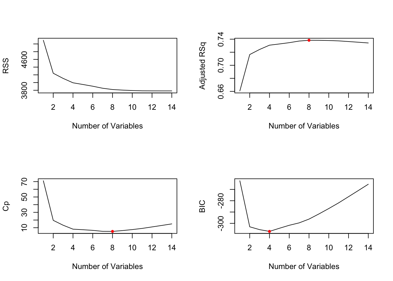
We see that the measures are not in sync with one another and we realise that no one measure is going to give us an entirely accurate picture. According to \(\bar{R}^2\) and \(C_p\) the best performing model is the one with 8 variables and according to \(BIC\) the best performing model has only 4 variables. This outcome suggests that the models with fewer than 4 predictors is insufficient, while a model with more than 8 predictors will overfit.
The regsubsets() function has a built-in plot() command which can be used to display the selected variables for the best model with a given number of predictors, ranked according to the \(R^2\), \(\bar{R}^2\), \(C_p\), and \(BIC\) statistic. The top row of each plot contains a black square for each variable selected according to the optimal model associated with that statistic. That is, when creating this plot for the display of the \(R^2\) value it is not a surprise to see that the top row indicates inclusion of all 14 predictors for the \(R^2\) of 75%.
plot(breg_full, scale="r2")
We can now identify the suggested 8 predictors for the best model by observing the top row and checking which of the variables has a black square.
In the following plot by observing the top row and checking which of the variable has a black square we can identify the exact 8 predictors to be used for the best model as suggested by \(\bar{R}^2\).
plot(breg_full, scale ="adjr2") It suggests that \[brozek = f(age, weight, neck, abdom, hip, thigh, forearm, wrist)\]
We can use the
It suggests that \[brozek = f(age, weight, neck, abdom, hip, thigh, forearm, wrist)\]
We can use the coef() function to see the coefficient estimates associated with this model.
coef(breg_full, 8)## (Intercept) age weight neck abdom hip
## -20.06213373 0.05921577 -0.08413521 -0.43189267 0.87720667 -0.18641032
## thigh forearm wrist
## 0.28644340 0.48254563 -1.40486912plot(breg_full, scale="Cp")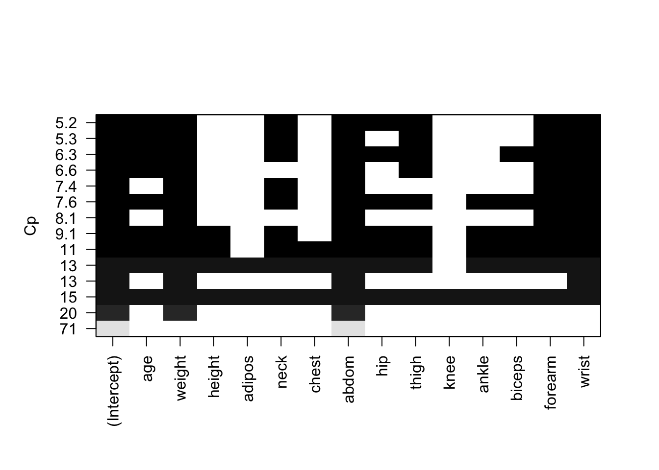
\(C_p\) suggests the same set of predictors as \(\bar{R}^2\).
plot(breg_full, scale="bic")
We see that two models share a BIC close to -310. However, the model with the lowest \(BIC\) is the four-variable model that contains only weight, abdom, forearm and wrist
coef(breg_full, 4)## (Intercept) weight abdom forearm wrist
## -31.2967858 -0.1255654 0.9213725 0.4463824 -1.3917662Forward and Backward Stepwise Selection
To perform stepwise selection we will also use the regsubsets() function, but this time with the argument method set to either “forward” or “backward” depending on which of the two stepwise selections we wish to perform.
# Forward stepwise selection
stepw_fwd <- regsubsets(brozek ~ ., data = bodyfat, nvmax = 14, method = "forward")
summary(stepw_fwd)
## Subset selection object
## Call: regsubsets.formula(brozek ~ ., data = bodyfat, nvmax = 14, method = "forward")
## 14 Variables (and intercept)
## Forced in Forced out
## age FALSE FALSE
## weight FALSE FALSE
## height FALSE FALSE
## adipos FALSE FALSE
## neck FALSE FALSE
## chest FALSE FALSE
## abdom FALSE FALSE
## hip FALSE FALSE
## thigh FALSE FALSE
## knee FALSE FALSE
## ankle FALSE FALSE
## biceps FALSE FALSE
## forearm FALSE FALSE
## wrist FALSE FALSE
## 1 subsets of each size up to 14
## Selection Algorithm: forward
## age weight height adipos neck chest abdom hip thigh knee ankle biceps
## 1 ( 1 ) " " " " " " " " " " " " "*" " " " " " " " " " "
## 2 ( 1 ) " " "*" " " " " " " " " "*" " " " " " " " " " "
## 3 ( 1 ) " " "*" " " " " " " " " "*" " " " " " " " " " "
## 4 ( 1 ) " " "*" " " " " " " " " "*" " " " " " " " " " "
## 5 ( 1 ) " " "*" " " " " "*" " " "*" " " " " " " " " " "
## 6 ( 1 ) "*" "*" " " " " "*" " " "*" " " " " " " " " " "
## 7 ( 1 ) "*" "*" " " " " "*" " " "*" " " "*" " " " " " "
## 8 ( 1 ) "*" "*" " " " " "*" " " "*" "*" "*" " " " " " "
## 9 ( 1 ) "*" "*" " " " " "*" " " "*" "*" "*" " " " " "*"
## 10 ( 1 ) "*" "*" " " " " "*" " " "*" "*" "*" " " "*" "*"
## 11 ( 1 ) "*" "*" "*" " " "*" " " "*" "*" "*" " " "*" "*"
## 12 ( 1 ) "*" "*" "*" " " "*" "*" "*" "*" "*" " " "*" "*"
## 13 ( 1 ) "*" "*" "*" "*" "*" "*" "*" "*" "*" " " "*" "*"
## 14 ( 1 ) "*" "*" "*" "*" "*" "*" "*" "*" "*" "*" "*" "*"
## forearm wrist
## 1 ( 1 ) " " " "
## 2 ( 1 ) " " " "
## 3 ( 1 ) " " "*"
## 4 ( 1 ) "*" "*"
## 5 ( 1 ) "*" "*"
## 6 ( 1 ) "*" "*"
## 7 ( 1 ) "*" "*"
## 8 ( 1 ) "*" "*"
## 9 ( 1 ) "*" "*"
## 10 ( 1 ) "*" "*"
## 11 ( 1 ) "*" "*"
## 12 ( 1 ) "*" "*"
## 13 ( 1 ) "*" "*"
## 14 ( 1 ) "*" "*"stepw_bwd <- regsubsets(brozek ~ ., data = bodyfat, nvmax = 14, method = "backward")
summary(stepw_bwd)## Subset selection object
## Call: regsubsets.formula(brozek ~ ., data = bodyfat, nvmax = 14, method = "backward")
## 14 Variables (and intercept)
## Forced in Forced out
## age FALSE FALSE
## weight FALSE FALSE
## height FALSE FALSE
## adipos FALSE FALSE
## neck FALSE FALSE
## chest FALSE FALSE
## abdom FALSE FALSE
## hip FALSE FALSE
## thigh FALSE FALSE
## knee FALSE FALSE
## ankle FALSE FALSE
## biceps FALSE FALSE
## forearm FALSE FALSE
## wrist FALSE FALSE
## 1 subsets of each size up to 14
## Selection Algorithm: backward
## age weight height adipos neck chest abdom hip thigh knee ankle biceps
## 1 ( 1 ) " " " " " " " " " " " " "*" " " " " " " " " " "
## 2 ( 1 ) " " "*" " " " " " " " " "*" " " " " " " " " " "
## 3 ( 1 ) " " "*" " " " " " " " " "*" " " " " " " " " " "
## 4 ( 1 ) " " "*" " " " " " " " " "*" " " " " " " " " " "
## 5 ( 1 ) "*" "*" " " " " " " " " "*" " " " " " " " " " "
## 6 ( 1 ) "*" "*" " " " " " " " " "*" " " "*" " " " " " "
## 7 ( 1 ) "*" "*" " " " " "*" " " "*" " " "*" " " " " " "
## 8 ( 1 ) "*" "*" " " " " "*" " " "*" "*" "*" " " " " " "
## 9 ( 1 ) "*" "*" " " " " "*" " " "*" "*" "*" " " " " "*"
## 10 ( 1 ) "*" "*" " " " " "*" " " "*" "*" "*" " " "*" "*"
## 11 ( 1 ) "*" "*" "*" " " "*" " " "*" "*" "*" " " "*" "*"
## 12 ( 1 ) "*" "*" "*" " " "*" "*" "*" "*" "*" " " "*" "*"
## 13 ( 1 ) "*" "*" "*" "*" "*" "*" "*" "*" "*" " " "*" "*"
## 14 ( 1 ) "*" "*" "*" "*" "*" "*" "*" "*" "*" "*" "*" "*"
## forearm wrist
## 1 ( 1 ) " " " "
## 2 ( 1 ) " " " "
## 3 ( 1 ) " " "*"
## 4 ( 1 ) "*" "*"
## 5 ( 1 ) "*" "*"
## 6 ( 1 ) "*" "*"
## 7 ( 1 ) "*" "*"
## 8 ( 1 ) "*" "*"
## 9 ( 1 ) "*" "*"
## 10 ( 1 ) "*" "*"
## 11 ( 1 ) "*" "*"
## 12 ( 1 ) "*" "*"
## 13 ( 1 ) "*" "*"
## 14 ( 1 ) "*" "*"stepw_new <- regsubsets(brozek ~ ., data = bodyfat, nvmax = 14, method = "seqrep")
summary(stepw_new)## Subset selection object
## Call: regsubsets.formula(brozek ~ ., data = bodyfat, nvmax = 14, method = "seqrep")
## 14 Variables (and intercept)
## Forced in Forced out
## age FALSE FALSE
## weight FALSE FALSE
## height FALSE FALSE
## adipos FALSE FALSE
## neck FALSE FALSE
## chest FALSE FALSE
## abdom FALSE FALSE
## hip FALSE FALSE
## thigh FALSE FALSE
## knee FALSE FALSE
## ankle FALSE FALSE
## biceps FALSE FALSE
## forearm FALSE FALSE
## wrist FALSE FALSE
## 1 subsets of each size up to 14
## Selection Algorithm: 'sequential replacement'
## age weight height adipos neck chest abdom hip thigh knee ankle biceps
## 1 ( 1 ) " " " " " " " " " " " " "*" " " " " " " " " " "
## 2 ( 1 ) " " "*" " " " " " " " " "*" " " " " " " " " " "
## 3 ( 1 ) " " "*" " " " " " " " " "*" " " " " " " " " " "
## 4 ( 1 ) " " "*" " " " " " " " " "*" " " " " " " " " " "
## 5 ( 1 ) " " "*" " " " " "*" " " "*" " " " " " " " " " "
## 6 ( 1 ) "*" "*" " " " " " " " " "*" " " "*" " " " " " "
## 7 ( 1 ) "*" "*" "*" "*" "*" "*" "*" " " " " " " " " " "
## 8 ( 1 ) "*" "*" " " " " "*" " " "*" "*" "*" " " " " " "
## 9 ( 1 ) "*" "*" " " " " "*" " " "*" "*" "*" " " " " "*"
## 10 ( 1 ) "*" "*" " " " " "*" " " "*" "*" "*" " " "*" "*"
## 11 ( 1 ) "*" "*" "*" "*" "*" "*" "*" "*" "*" "*" "*" " "
## 12 ( 1 ) "*" "*" "*" " " "*" "*" "*" "*" "*" " " "*" "*"
## 13 ( 1 ) "*" "*" "*" "*" "*" "*" "*" "*" "*" "*" "*" "*"
## 14 ( 1 ) "*" "*" "*" "*" "*" "*" "*" "*" "*" "*" "*" "*"
## forearm wrist
## 1 ( 1 ) " " " "
## 2 ( 1 ) " " " "
## 3 ( 1 ) " " "*"
## 4 ( 1 ) "*" "*"
## 5 ( 1 ) "*" "*"
## 6 ( 1 ) "*" "*"
## 7 ( 1 ) " " " "
## 8 ( 1 ) "*" "*"
## 9 ( 1 ) "*" "*"
## 10 ( 1 ) "*" "*"
## 11 ( 1 ) " " " "
## 12 ( 1 ) "*" "*"
## 13 ( 1 ) "*" " "
## 14 ( 1 ) "*" "*"We can see that the best one-variable through four-variable models are each identical for best subset and forward and backward selection. Difference occurs for the five-variable model for which the backward selection method selects different set of predictors from the other two.
coef(breg_full, 5)## (Intercept) weight neck abdom forearm wrist
## -27.4118045 -0.1136977 -0.3382162 0.9325574 0.4964234 -1.1519642coef(stepw_fwd, 5)## (Intercept) weight neck abdom forearm wrist
## -27.4118045 -0.1136977 -0.3382162 0.9325574 0.4964234 -1.1519642coef(stepw_bwd, 5)## (Intercept) age weight abdom forearm wrist
## -27.89197896 0.03594628 -0.10392579 0.87162722 0.47755107 -1.67587889Another difference in selection happens again for the six-factor model for which this time forward selection suggests a different set of predictors from the other two.
coef(breg_full, 6)## (Intercept) age weight abdom thigh forearm
## -34.8393955 0.0566420 -0.1280528 0.8459061 0.2081457 0.4592612
## wrist
## -1.6278694coef(stepw_fwd, 6)## (Intercept) age weight neck abdom forearm
## -23.21489668 0.04059830 -0.08818394 -0.36881380 0.87738614 0.53615286
## wrist
## -1.45115127coef(stepw_bwd, 6)## (Intercept) age weight abdom thigh forearm
## -34.8393955 0.0566420 -0.1280528 0.8459061 0.2081457 0.4592612
## wrist
## -1.6278694For the models with seven predictors and more all three methods suggest the same variables.
The Validation Set Approach and Cross-Validation for the selection of the best model
In this section validation set and cross-validation approaches will be used to chose the best model among a set of models of different sizes. When applying these approaches we split the given data into two subsets:
- training data: a subset to train a model
- test data: a subset to test the model
The training data is used for model estimation and variable selection, whilst the remaining test data is put aside and reserved for testing the accuracy of the model (see section on Machine Learning). That is, the best model variable selection is performed using only the training observations that are randomly selected from the original data.
We begin the application of validation approach in R by splitting the bodyaft data into a training set and a test set. First, we set a random seed to ensure the same data split each time we run the randomised process of splitting the bodyfat data into training set and test set. The set.seed() function sets the starting number used to generate a sequence of random numbers (it ensures that you get the same result if you start with that same seed each time you run the same process). Next, we create a random vector, train, of elements equal to TRUE if the corresponding observation is in the training set, and FALSE otherwise. A random vector test is obtained by using the ! command that creates TRUEs to be switched to FALSEs and vice versa. Once both train and test vectors are obtained we perform best subset on the training set of the bodyfat data using the now familiar regsubset() function.
set.seed(111)
train <- sample(c(TRUE, FALSE), nrow(bodyfat), rep = TRUE)
test <- (!train )
breg <- regsubsets(brozek ~., data = bodyfat[train, ], nvmax = 14)
We now compute the validation set error for the best model of each model size. We first make a model matrix from the test data. The model.matrix() function is used in many regression packages for building an \(X\) matrix from data.
In the multiple regression setting because of the potentially large number of predictors, it is more convenient to write the expressions using matrix notation. To develop the analogy let us quickly look at the matrix notation for the 14-variable linear regression function:
\[y_i = \beta_0 + \beta_1x_1 + \epsilon_i \;\;\;\;\;\; \text{for} \;\; i=1, 2, ...n\] If we actually let \(i = 1, ..., n\), we see that we obtain \(n\) equations: \[y_i = \beta_0 + \beta_1x_1 + \epsilon_1\] \[y_i = \beta_0 + \beta_1x_2 + \epsilon_2\] \[ \vdots\] \[y_i = \beta_0 + \beta_1x_n + \epsilon_n\] It is more efficient to use matrices to define the regression model which can be formulated for the above simple linear regression function in matrix notation as: \[ \begin{bmatrix} y_1\\y_2\\ \vdots\\y_n \end{bmatrix} = \begin{bmatrix} 1 & x_1 \\ 1 & x_2 \\ \vdots & \vdots \\ 1 & x_n \\ \end{bmatrix} \begin{bmatrix} \beta_0\\\beta_1\\ \end{bmatrix} + \begin{bmatrix} \varepsilon_1\\\varepsilon_2\\ \vdots\\\varepsilon_n \end{bmatrix} \] Instead of writing out the \(n\) equations, using matrix notation, the simple linear regression function reduces to a short and simple statement: \[\mathbf{Y} = \mathbf{X\beta} + \mathbf{\varepsilon},\] where matrices \(Y\), \(\mathbf{\varepsilon}\) are of the size \(n \times 1\), \(\mathbf{\beta}\) of \(2 \times 1\) and finally matrix \(Y\) of \(n \times 2\).
Once we have created \(X\) matrix we run a loop, and for each \(i\), we
- extract the coefficients from
bregfor the best model of that size - multiply them into the appropriate columns of the test model matrix to form the predictions and
- compute the test MSE
test.mat <- model.matrix(brozek ~., data = bodyfat[test, ])
val.errors <- rep(NA, 14)
for(i in 1:14){
 coefi <- coef(breg, id = i)
 pred <- test.mat[ ,names(coefi)] %*% coefi
 val.errors[i] <- mean((bodyfat$brozek[test] - pred)^2)
}
val.errors
## [1] 20.43699 16.90849 16.75413 16.20119 16.04250 17.82335 17.46721 17.64863
## [9] 17.55764 17.06395 16.60744 17.00481 16.94781 16.84543coef(breg, which.min(val.errors))## (Intercept) weight neck abdom forearm wrist
## -25.45466859 -0.09711483 -0.39312889 0.95767906 0.38200504 -1.25643570It looks as if the best model is the one that contains five variables. As there is no predict() method for regsubsets() we can capture our steps above and write our own predict method.
predict.regsubsets <- function(object, newdata, id,...){
 form <- as.formula(object$call[[2]])
 mat <- model.matrix(form, newdata)
 coefi <- coef(object, id = id)
 xvars <- names(coefi)
 mat[,xvars ] %*% coefi
 }
The function almost does what we did above. The only tricky bit is the extraction of the formula used in the call to regsubsets(). We are going to use this function to do cross-validation. We start by performing best subset selection on the full data set, and select the best five-variable model. In order to get more accurate coefficient estimates we make use of the full data set, rather than using the variables that were obtained from the training set. We should realise that the best five-variable model on the full data set may differ from the corresponding five-variable model on the training set.
breg <- regsubsets(brozek ~., data = bodyfat , nvmax = 14)
coef(breg, 5)
## (Intercept) weight neck abdom forearm wrist
## -27.4118045 -0.1136977 -0.3382162 0.9325574 0.4964234 -1.1519642We are in luck as the best five-variable model on the full data set has the same set of variables as identified for the best five-variable model on the training set.
We now try to choose among the models of different sizes using cross-validation and perform best subset selection within each of the \(k\) training sets. This taxing task can be easily performed in R by creating a vector that allocates each observation to one of k = 10 folds and a matrix that will hold the results.
k <- 10
set.seed(111)
folds <- sample (1:k, nrow(bodyfat), replace = TRUE)
cv.errors <- matrix(NA, k, 14, dimnames = list(NULL, paste (1:14)))
Now we write a for loop that performs cross-validation:
- in the \(j^{\text{th}}\) fold, the elements of folds that equal \(j\) are in the test set, and the remainder are in the training set.
- next,
- make our predictions for each model size (using our new
predict()method) - compute the test errors on the appropriate subset, and
- store them in the appropriate slot in the matrix
cv.errors.
for(j in 1:k){
 best.fit <- regsubsets(brozek ~., data = bodyfat[folds!=j, ], nvmax = 14)
 for(i in 1:14){
    pred <- predict(best.fit, bodyfat[folds==j, ], id = i)
    cv.errors[j, i] <- mean((bodyfat$brozek[folds==j] - pred)^2)
 }
}
This creates a 10 \(\times\) 14 matrix, where the \((i, j)^{\text{th}}\) element represents the test MSE for the \(i^{\text{th}}\) cross-validation fold for the best \(j\)-variable model. We use apply() to average over the columns of this matrix in order to obtain a vector for which the \(j^{\text{th}}\) element is the cross-validation error for the \(j\)-variable model.
mean.cv.errors <- apply(cv.errors, 2,  mean)
mean.cv.errors
## 1 2 3 4 5 6 7 8
## 20.34108 17.51758 17.10110 17.13365 17.53639 17.85260 17.54328 17.54522
## 9 10 11 12 13 14
## 31.93117 35.00292 35.25575 34.60876 34.99476 34.96073cv.errors## 1 2 3 4 5 6 7 8
## [1,] 12.32946 9.416819 9.903653 11.10810 12.19012 13.10063 13.37630 13.56035
## [2,] 12.48594 13.771297 13.852726 12.72790 12.99102 13.28162 13.21003 13.36145
## [3,] 15.55276 13.954025 14.715055 14.75803 15.87441 14.79482 15.16436 13.98156
## [4,] 31.60131 23.661676 21.820352 20.87529 22.30423 22.44055 23.90745 22.11288
## [5,] 21.10524 24.206510 21.984589 21.35164 22.34848 23.97423 20.04423 20.86420
## [6,] 21.92108 16.523561 16.195050 15.11413 15.57349 15.48747 14.61914 14.04020
## [7,] 19.97793 21.266331 20.512493 20.99681 20.69149 20.58539 20.26534 19.82136
## [8,] 17.86496 12.694993 12.796383 13.62946 13.55600 13.63481 12.65788 12.28301
## [9,] 15.83071 15.834488 14.922103 15.21815 14.95377 15.17270 14.62951 15.25427
## [10,] 34.74140 23.846053 24.308575 25.55695 24.88093 26.05378 27.55856 30.17297
## 9 10 11 12 13 14
## [1,] 13.60245 13.58774 13.41241 13.46334 13.44878 13.45282
## [2,] 14.11558 14.21637 13.99672 13.94406 14.02302 13.99533
## [3,] 14.09255 13.99584 14.08496 14.16646 14.69319 14.91532
## [4,] 22.23907 21.92254 22.40096 22.45297 22.49736 22.50527
## [5,] 165.51126 197.37461 200.09727 193.90667 196.86868 196.97994
## [6,] 13.87184 13.77324 13.69918 13.80556 13.97567 13.98346
## [7,] 19.94554 20.10140 20.08304 20.15145 20.17206 20.19522
## [8,] 12.32055 12.29925 12.06850 12.06478 12.04933 12.05878
## [9,] 15.56205 15.55901 15.21091 15.30418 15.32023 15.32022
## [10,] 28.05086 27.19924 27.50356 26.82817 26.89926 26.20099par(mfrow=c(1, 1))
plot(mean.cv.errors, type="b")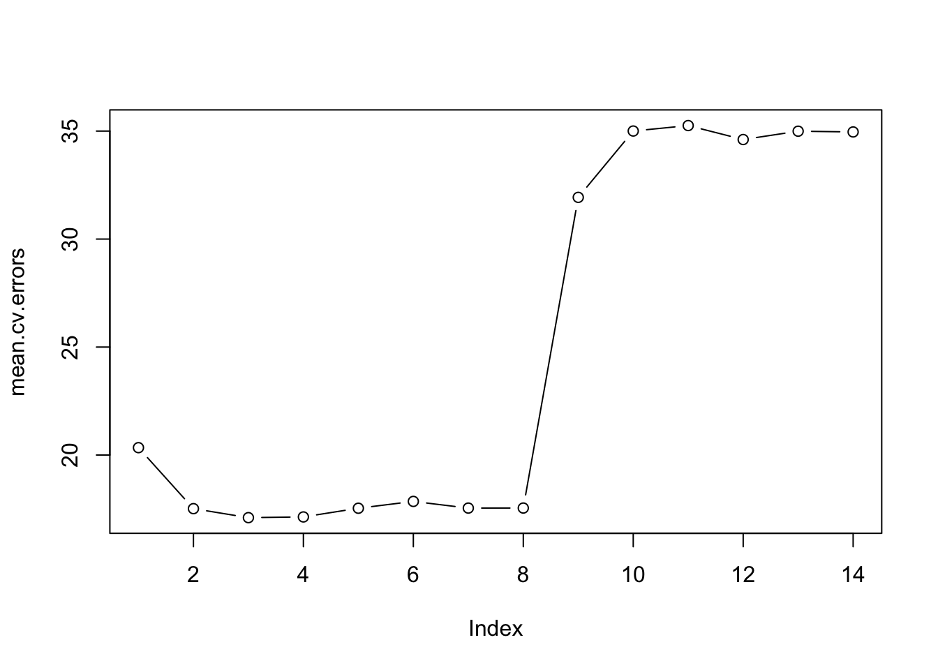
We see that cross-validation selects a three-variable model. We will use breg_full in order to obtain the three-variable model.
#breg <- regsubsets(brozek ~., data = bodyfat, nvmax = 4)
coef(breg_full, 3)
## (Intercept) weight abdom wrist
## -24.7612893 -0.1055832 0.9019083 -1.1456968
caret: Stepwise and Cross-Validation put together
The caret package makes modelling in R easier. It combines two in one:
- automatically resamples the models
- while conducting parameter tuning
caret’s most affable feature is its consistent modelling syntax which enables you to build and compare models with very little splurge. By simply changing the method argument, you can easily investigate varying applicable models adopted from the pre-existing R packages. In total there are over two hundred different models available in caret.
Another sublime feature of caret lies in its train() function, which enables the use of the same function to run all of the competing models. It accepts several caret-specific arguments that provide capabilities for different resampling methods, performance measures, and algorithms for choosing the best model. Running the train() function will create a train object with estimated parameters for a selected model from a set of given data with many other useful results.
We will use caret to adopt 10-fold cross-validation, that will split bodyfat data into 10 approximately equal chunks to perform stepwise selections using the leapBackward method adopted from the leaps package.
The model will be developed based on 9 chunks and predict the \(\text{$10^{th}$}\) until all of the folds are treated as a validation set, while the model is fitted on the remaining 10-1 folds. caret takes care of setting up this resampling with the help of the trainControl() function and the trControl argument of its train() function. As the data set contains 14 predictors, we will vary nvmax from 1 to 14 resulting in the identification of the 14 best models with different sizes: the best 1-variable model, the best 2-variables model, and so on up to the best 14-variables model.
#If you don't have the "caret" package installed yet, uncomment and run the line below
#install.packages("caret")
# Train the model
suppressPackageStartupMessages(library(caret))
set.seed(111)
# Set up repeated k-fold cross-validation
train.control <- trainControl(method = "cv", number = 10)
# Train the model
stepwb <- train(brozek ~., data = bodyfat,
                    method = "leapBackward",
                    tuneGrid = data.frame(nvmax = 1:14),
                    trControl = train.control
                    )
class(stepwb)
## [1] "train" "train.formula"stepwb$results## nvmax RMSE Rsquared MAE RMSESD RsquaredSD MAESD
## 1 1 4.500901 0.6779062 3.667717 0.8055119 0.11240896 0.5675990
## 2 2 4.260896 0.7022554 3.501954 0.7003423 0.11479575 0.6140745
## 3 3 4.257837 0.7103567 3.493261 0.6797350 0.09896541 0.5393138
## 4 4 4.173503 0.7218316 3.444086 0.6125089 0.09224353 0.5335659
## 5 5 4.227939 0.7159505 3.511170 0.6146446 0.08503459 0.5306893
## 6 6 4.186677 0.7200482 3.465637 0.6156029 0.08406015 0.5571481
## 7 7 4.139519 0.7272454 3.387318 0.6905944 0.08203603 0.5906919
## 8 8 4.130202 0.7290699 3.379290 0.6346024 0.07918020 0.5620786
## 9 9 4.138647 0.7279039 3.397510 0.6191154 0.08006510 0.5422292
## 10 10 4.151920 0.7245898 3.410971 0.6212871 0.08515454 0.5505494
## 11 11 4.140745 0.7268756 3.396724 0.6400128 0.08463738 0.5612896
## 12 12 4.183797 0.7214162 3.423895 0.6614864 0.08789564 0.5794326
## 13 13 4.196041 0.7197241 3.434989 0.6747641 0.09008652 0.5887054
## 14 14 4.199835 0.7192288 3.437822 0.6768053 0.09037830 0.5945132The output above shows different metrics and their standard deviation for comparing the accuracy of the 14 best models for a different number of variables.
nvmax: the number of variables; in the best model for the given number of variablesRMSEandMAEare two different metrics measuring the prediction error of the model, implying that the lower their value, the better the model.Rsquaredindicates the correlation between the observed outcome values and the values predicted by the model, meaning that the higher theRsquared, the better the model.
Using the 10-fold cross-validation we have estimated average prediction error (RMSE) for each of the 14 best models for the given number of variables. The RMSE statistical metric is used to compare the 14 selected models and to automatically choose the model that minimises the RMSE as the best model. It can be seen that the model with 8 variables (nvmax = 8) is the one that has the lowest RMSE. We can call bestTune from the created stepwb object of class train to directly display the “best tuning values” (nvmax) and finalModel to see selected variables of the best model.
# Final model coefficients
stepwb$finalModel
## Subset selection object
## 14 Variables (and intercept)
## Forced in Forced out
## age FALSE FALSE
## weight FALSE FALSE
## height FALSE FALSE
## adipos FALSE FALSE
## neck FALSE FALSE
## chest FALSE FALSE
## abdom FALSE FALSE
## hip FALSE FALSE
## thigh FALSE FALSE
## knee FALSE FALSE
## ankle FALSE FALSE
## biceps FALSE FALSE
## forearm FALSE FALSE
## wrist FALSE FALSE
## 1 subsets of each size up to 8
## Selection Algorithm: backward# Summary of the model
stepwb$bestTune## nvmax
## 8 8summary(stepwb$finalModel)## Subset selection object
## 14 Variables (and intercept)
## Forced in Forced out
## age FALSE FALSE
## weight FALSE FALSE
## height FALSE FALSE
## adipos FALSE FALSE
## neck FALSE FALSE
## chest FALSE FALSE
## abdom FALSE FALSE
## hip FALSE FALSE
## thigh FALSE FALSE
## knee FALSE FALSE
## ankle FALSE FALSE
## biceps FALSE FALSE
## forearm FALSE FALSE
## wrist FALSE FALSE
## 1 subsets of each size up to 8
## Selection Algorithm: backward
## age weight height adipos neck chest abdom hip thigh knee ankle biceps
## 1 ( 1 ) " " " " " " " " " " " " "*" " " " " " " " " " "
## 2 ( 1 ) " " "*" " " " " " " " " "*" " " " " " " " " " "
## 3 ( 1 ) " " "*" " " " " " " " " "*" " " " " " " " " " "
## 4 ( 1 ) " " "*" " " " " " " " " "*" " " " " " " " " " "
## 5 ( 1 ) "*" "*" " " " " " " " " "*" " " " " " " " " " "
## 6 ( 1 ) "*" "*" " " " " " " " " "*" " " "*" " " " " " "
## 7 ( 1 ) "*" "*" " " " " "*" " " "*" " " "*" " " " " " "
## 8 ( 1 ) "*" "*" " " " " "*" " " "*" "*" "*" " " " " " "
## forearm wrist
## 1 ( 1 ) " " " "
## 2 ( 1 ) " " " "
## 3 ( 1 ) " " "*"
## 4 ( 1 ) "*" "*"
## 5 ( 1 ) "*" "*"
## 6 ( 1 ) "*" "*"
## 7 ( 1 ) "*" "*"
## 8 ( 1 ) "*" "*"💡Typing ?caret::train inside R’s console will bring a more detailed explanation on how to use the train() function and information about the expected outcomes.
Summary
All of the above approaches have suggested different variable selection for the best fitted model. We have noticed by examining the correlogram high multicollinearity amongst the variables in the bodyfat. It reveals a weak correlation only between three to four variables. This is a frequently encountered problem in multiple regression analysis, where such an interrelationship among explanatory variables obscures their relationship with the response variable. This causes computational instability in model estimation resulting in the different suggestions of the best model for different variable selection approaches:
- Best Subsets Regression: has indicated that the models with a fewer than 4 predictors is insufficient, while a model with more than 8 predictors will overfit
- Stepwise Forward and Stepwise Backward selections: has suggested different sets of variables for the five-factor model and the six-factor model
- Validation Set: has recommended the five-factor model as the best one
- 10-Fold Cross-Validation: has argued the case for the three-factor model
- Backward Selection with automatic 10-Fold Cross-Validation adopted by the application of the
caretpackage: identifies the eight-factor model as the best one
Our main goal was to derive a model to predict body fat (variable brozek) using all predictors except for siri, density and free from the fat data available from the faraway package. Guided by the outcomes of the above analysis and a desire to describe the behaviour of this multivariate data set parsimoniously (see Miller, 2002) we suggest the four-factor model for which \(\bar{R}^2\) = 73.51%. Adding another 4 variables as suggested by Backward Selection with automatic 10-Fold Cross-Validation would increase \(\bar{R}^2\) statistic by only 1.16%.
coef(breg_full, 4)## (Intercept) weight abdom forearm wrist
## -31.2967858 -0.1255654 0.9213725 0.4463824 -1.3917662\[brozek = -31.2967858 - 0.1255654 \; weight + 0.9213725 \; abdom + 0.4463824 \; forearm - 1.3917662 \; wrist\] Applying different subset selection approaches we have pruned a list of plausible explanatory variables down to a parsimonious collection of the “most useful” variables. We need to realise that subset selection approaches for multiple regression modelling should be used as a tool that can help us avoid the tiresome process of trying all possible combinations of explanatory variables, by testing variables one by one. However, as statistical models can serve different purposes we need to incorporate prior knowledge when it is possible. Solely reliance on subset selection approaches is wrong and it could be misleading (Smith, 2018).
YOUR TURN 👇
Practise by doing the following exercises:
- Use multiple regression on the Air Quality Data data set.
Produce a correlogram which include all the variables in the data set.
Use the
lm()function to perform multiple regression withOzoneas the response and all other variables as the predictors. Use thesummary()function to print the results and comment on the output, in particular:- is there a relationship between the predictors and the response, i.e. is the model valid?
- which predictors appear to have a statistically significant relationship to the response?
- on the basis of your response to the previous question, fit a smaller model that only uses predictors for which there is evidence of association with the response variable.
Try out some of the variable selection methods explained in this section. Present and discuss the results from the chosen approach(es).
Propose with justification a model (or a set of models) that seem to perform well on this data set. Make sure you provide justified explanation on the selected set of predictors in the proposed model.
M. Friendly. Corrgrams: Exploratory displays for correlation matrices, The American Statistician 56(4): 316-324, 2002.
M. Kuhn. The caret Package, 2019.
A. J. Miller. Subset Selection in Regression. Monographs on Statistics and Applied Probability, Chapman & Hall/CRC, 2\(^\text{nd}\) edition, 2002.
G. Smith. Step away from stepwise. Journal of Big Data, 5-32. 2018
© 2020 Tatjana Kecojevic