Resampling

We use resampling techniques for estimating model performance. In the previous section we presented the idea of fitting a model on a subset of data, known as tanning data and using the remaining sample, better known as test data, to assess the efficiency of the model. Often, this process is repeated multiple times and the results are aggregated and summarized. Hence, resampling method involves repeatedly drawing samples from a training data set and refitting a model to obtain addition information about that model.

Resampling methods involve fitting the same statistical method multiple times using different subsets of the training data that can be computationally taxing. Fortunately, computing power has greatly advanced in the last few decades allowing for resampling techniques to become an indispensable tool of a statistical modelling procedure.

In general, resampling techniques differ in the way in which the subsets of data are chosen. We will consider the most commonly used resampling methods: cross-validation and bootstrap.

Cross-Validation: a refinement of the test set approach

When splitting data into training and test subsets it is possible that we can end up with a test subset that may not be representative of the overall population. As a consequence, the resulting model may appear to be highly accurate when it just happened to fit well on an atypical data set, and essentially it has poor accuracy when applied to future data.

Cross-Validation (CV), enables more assiduous accuracy checking of a model, as it is assessed on multiple different subsets of data, ensuring it will generalise well to data collected in the future. It is an extension of the training and test process that minimizes the sampling bias of machine learning models.

k-Fold Cross-Validation

This approach involves randomly dividing the set of observations into k groups, known as folds of approximately equal size.

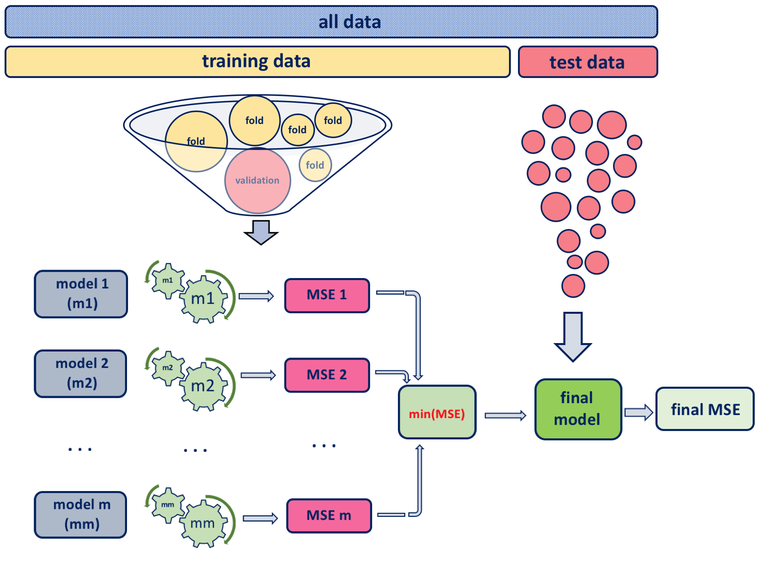
With cross-validation the test data is held out (approximately one fifth of data), and the remaining training data is randomly divided into \(k\) groups. Several different portions of this training data are used for validation, and the remaining part of the data is used for training as shown in the diagram below. Hence, a fold is treated as a validation set, and the method is fit on to the remaining \(k−1\) folds. The \(k\) resampled estimates of performance are summarized and used for testing and model building.

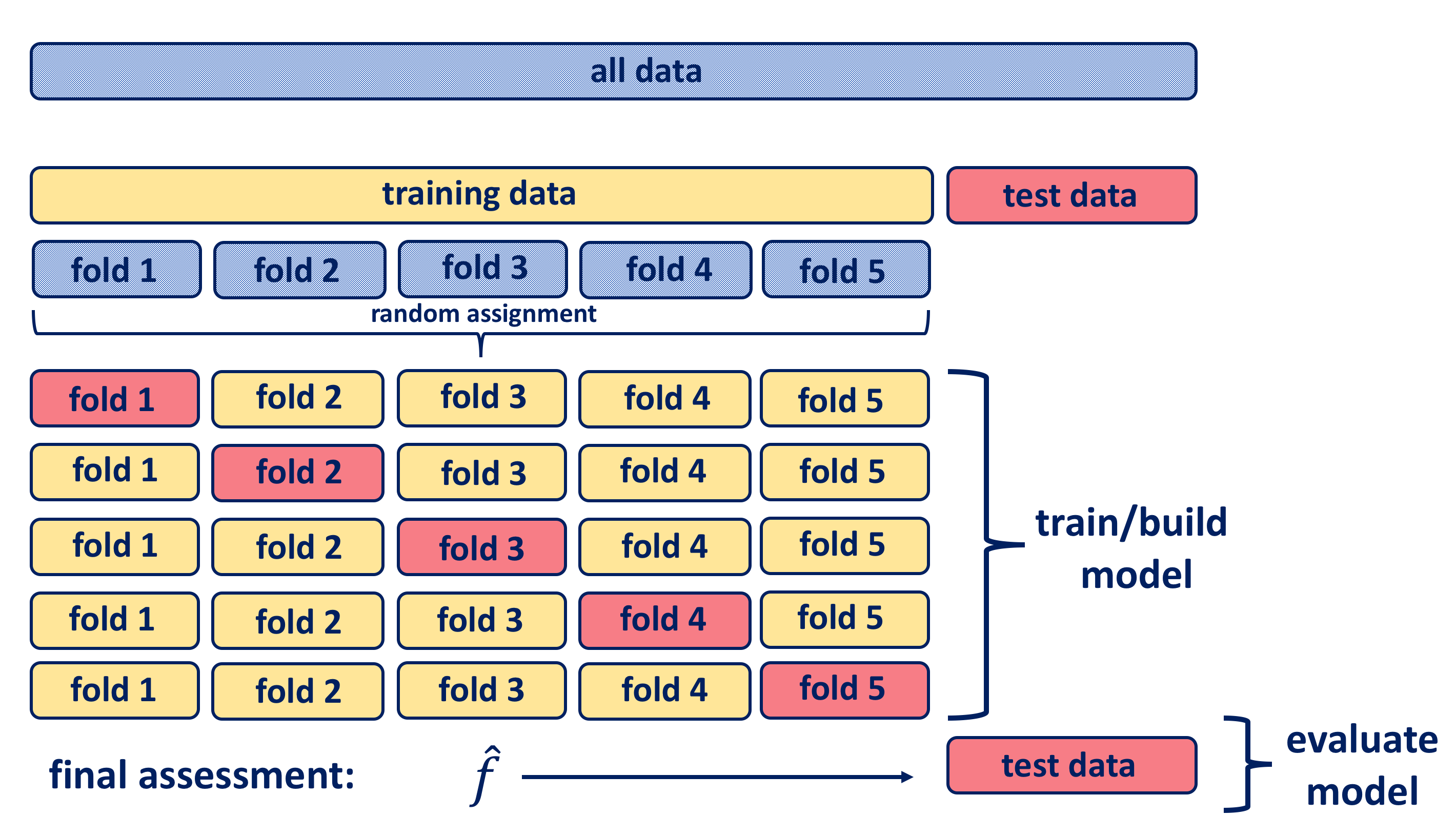
Since the non-holdout data is divided into five portions, we call this “5-fold cross-validation”. If there had been ten blocks, it would have been 10-fold cross-validation. The model that has been built using k-fold cross-validation is then tested on the originally held out test data subset. The \(k\) resampled estimates of model’s performance are summarized commonly using the mean and standard error to develop a better reasoning of its effectiveness in relation to its tuning parameters.

\[CV_{(k)} = \frac{1}{k}\sum^{k}_{i=1} MSE_{i}\]

A typical choice of \(k\) is \(5\) or \(10\), but there is no formal rule. One should keep in mind when making a choice that as \(k\) increases, the difference in size between the training set and the resampling subset gets smaller, causing the bias of the statistical model to become smaller.

Leave-One-Out Cross-Validation (LOOCV)

As in k-fold CV, the training set of data is split into two parts, with the difference that here they are not of comparable sizes as the validation set consists of a single observation and the remaining observations make up the training set.

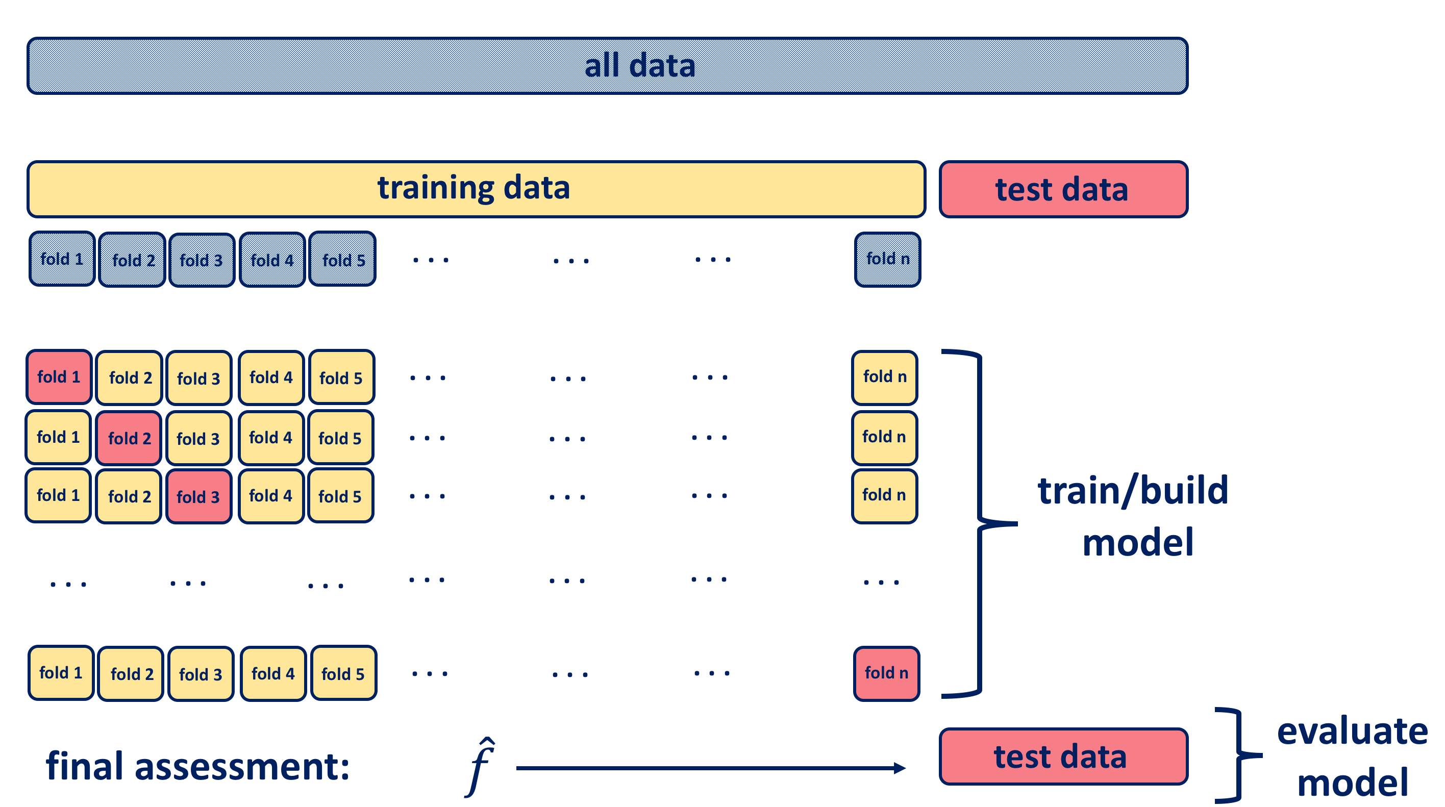
It is a special case of k-fold CV in which \(k\) is equal to \(n\). Repeating the process \(n\) times produces \(n\) square errors and the estimate for the test \(MSE\) is the average of those \(n\) test error estimates:

\[CV_{(n)} = \frac{1}{n}\sum^{n}_{i=1} MSE_{i}\]

The main advantage of the LOOCV approach over a simple train and test validation is that it produces less bias. The model is fit on \(n-1\) training observations, almost as many as there are in the entire data set. Furthermore, since LOOCV is performed multiple times it yields consistent results with less randomness than in a simple train and test approach. However, when compared with k-fold CV, LOOCV results in a poorer estimate as it provides an approximately unbiased estimate for the test error that is highly variable.

One more down side to the generally high value of \(k\) is that the computation side of the procedure becomes more taxing especially if the model is rather a complex one. Come to think about it, the LOOCV requires as many model fits as data points and each model fit uses a subset that is ALMOST the same size as the training.

Stratified K-Folds cross-validator

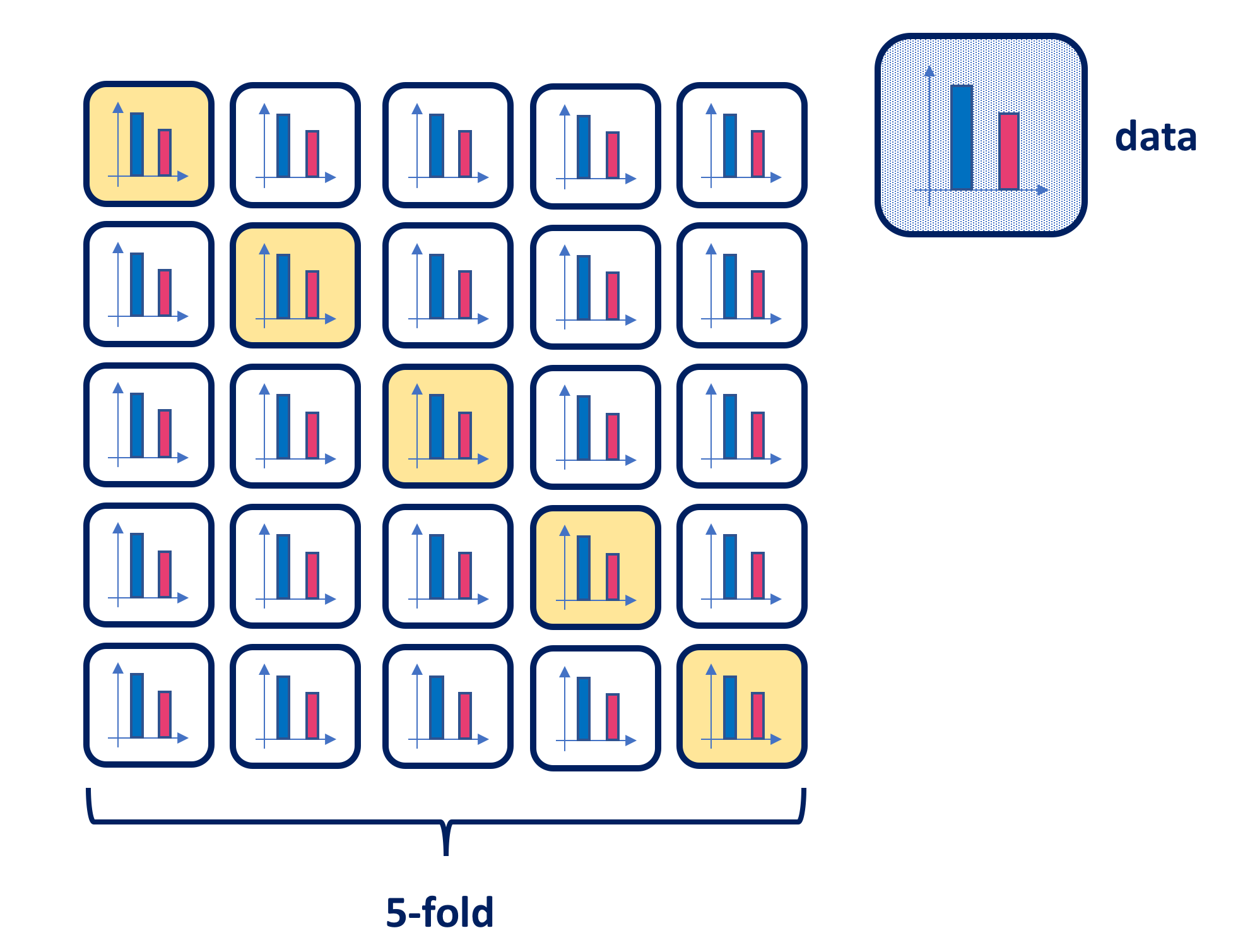
Another variation of k-fold CV is stratified k-fold CV, which returns stratified folds. This could be particularly useful for data that exhibit a large imbalance in the distribution of the target classes. As stratification is the process of rearranging the data in such a manner that each fold is a good representative of the whole, the stratified k-fold CV facilitates the preservation of the relative class frequencies in each train and validation fold. The figure below illustrates the process in the case of a binary classification.

Choice of \(k\)

Using k-fold cross-validation increases validation sensitivity, allowing better reasoning with the model. One of the key questions is how to choose the number of folds, i.e. how big does \(k\) need to be? In general, the choice of the number of folds depends on the size of the dataset. For large datasets 5-fold cross-validation is considered to be quite accurate and when dealing with very sparse datasets, we may consider using leave-one-out in order to train on as many examples as possible.

We have seen that there is a bias-variance trade-off associated with the choice of \(k\) in k-fold cross-validation. Larger \(k\), for which training folds are closer to the total dataset, results in less bias towards overestimating the true expected error but higher variance and higher running time. We can summarise those findings as follows:

• for a large number of folds
  • positives:
    1. small bias of the true error rate estimator (as a result of a very accurate estimator)
  • negatives:
    1. large variance of the true error rate estimator
    2. the computational time is large
• for a small number of folds
  • positives:
    1. small variance of the estimator
    2. the number of experiments and, therefore, computation time are reduced
  • negatives:
    1. large bias of the estimator

In practice, typical choises for \(k\) in cross-validation are \(k=5\) or \(k=10\), as these values have been shown empirically to yield test error rate estimates that suffer neither from excessively high bias nor from very high variance.

Bootstrap

The bootstrap method was introduced by Efron in 1979. Since then it has evolved considerably. Due to its intuitive nature, easily grasped by practitioners and available strong computational power necessary for its application, today bootstrapping is regarded as the indispensable tool for data analysis. The method is named after Baron Münchhausen, a fictional character who in one of the stories saved his life by pulling himself out of the bottom of a deep lake by his own hair.

Bootstrapping is a computationally intensive, nonparametric technique that makes probability-based inference about a population characteristic, \(\Theta\), based on an estimator, \(\hat\Theta\), using a sample drawn from a population. The data is resampled with replacement many times in order to obtain an empirical estimate of the sampling distribution of the statistic of interest \(\Theta\). Thus, bootstrapping enables us to make inference without having to make distributional assumptions (see Efron, 1979). In machine learning, for estimation purposes the idea of bootstrapping datasets has been proposed as an alternative to CV.

A bootstrap sample is a random sample of the data taken with replacement (Efron and Tibshirani 1986). Consequently, since samples are drawn with replacement, each bootstrap sample is likely to contain duplicate values. Bootstrapping relies on analogy between the sample and the population from which the sample was drawn, by treating the sample as if it is a population. The two key features of bootstrapping a sample with replacement are:

1. a data point is randomly selected for the subset and returned to the original data set, so that it is still available for further selection
2. the bootstrap sample is the same size as the original data set from which it was constructed

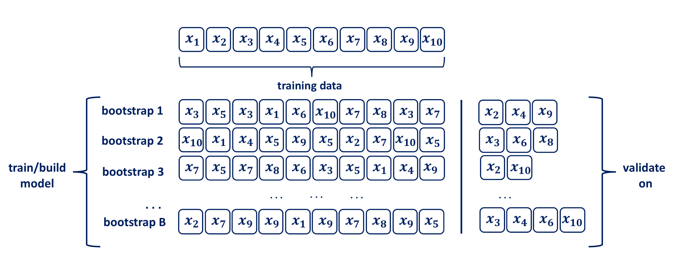
Using uniform re-sampling with replacement, a \(B\) number of training sets are produced by bootstrap to produce a performance estimate of a chosen statistical method, ie. model. The model is trained and its performance is estimated on the out-of-sample observations, as depicted in the figure above. The original observations not selected in a particular bootstrap sample are usually referred to as the out-of-bag (OOB). Hence, for a given bootstrap iteration, a model is built on the selected sample and is used to predict the out-of-bag sample. On average around \(63.2\%\) of the original sample ends up in any particular bootstrap sample (Mendelson et al. 2016).

When allying the bootstrapping procedure for inferential purposes typical chose for \(B\) is in the range of a few hundreds to thousands. Efron and Tibshirani (p.52) indicate that \(B=50\) and even \(B=25\) is usually sufficient for bootstrap standard error estimates and point out that there are rare occasions for which more than \(B=200\) replications are needed for estimating a standard error. In the context of using bootstraping for validation purposes the size of \(B\) in the range of hundreds may be unacceptably high, and the validation process should be repeated for a specified number of folds \(k\), i.e. set \(B=k\). Hence, the bootstrap resampling with replacement procedure for ML from a data set of size \(n\) can be summarised as follows:

1. randomly select with replacement \(n\) examples and use this set for training and model building
2. the remaining examples that were not selected for training are used for testing
3. repeat this process for a specific number of folds \(k\)
4. the true error is estimated as the average error rate on test examples

As Efron in his paper on etimating the error rates of prediction rules points out, when performing statistical modelling one might want more than just an estimate of an error rate. Bootstrap methods are helpful in understanding variability all aspects of the prediction problem. In this paper he makes comprehensive comparisons between different resampling methods, drawing the conclusion that in general the bootstrap error rates tend to have less uncertainty than k-fold cross-validation. One should also be aware that for small sample sizes the bias is noticeable and decreases as the sample size becomes larger as shown in Young and Daniels’ paper Bootsrap Bias.

Summary

The easiest way to assess the performance of a statistical method is by evaluating the error rate on a set of data that is independent of the training data. If model selection and true error estimates are to be computed simultaneously, the data should be divided into three disjointed sets as explained by Replay in his book.

In general we can summarise the ML model building procedure algorithm as follows:

1. divide the available data into training + validation and test sets
2. select model and training parameters
   1. train and build the model using the training set
   2. evaluate the model using the validation set
3. repeat step 2 using different model structures and tuning parameters
4. select the best model and train it using data from the training + validation set
5. assess this final model using the test set

When using cv or bootstrap sub-steps i) and ii) are repeated within step 2) for each of the \(k\) folds.

YOUR TURN 👇

1. Provide a rigorous explanation on how standard deviation of the prediction can be estimated for a statistical model that does prediction for the response \(Y\) for a particular value of the predictor \(X\). Identify the key steps and present them in an algorithmic manner.

© 2020 Tatjana Kecojevic