Data Literacy in R > Module 4 > Multiple Regression

Multiple Regression

In the previous section we learnt about simple linear regression as a very simple tool for predicting quantitative measured response variables. Its simple application, easy interpretation and predictive capabilities make it one of the most popular approaches for supervised learning. Developing good understanding of linear regression serves as a solid base for learning how to use and adopt other more sophisticated modelling procedures in the context of machine learning.

Additive Model

The basic idea in regression modelling is that there is a phenomenon of interest whose behaviour we seek to account for or explain. For example a company may be interested in why its sales figures have followed a particular pattern; Government officials may be interested in explaining the behaviour of unemployment statistics.

Let the phenomenon of interest be denoted by $Y$; as discussed in the previous sections, $Y$ is also known as the response variable, or the dependent variable. The fundamental nature of $Y$ is that it displays variability and it is this inherent variability that the data analyst seeks to explain by using regression modelling. Intuitively, if we can account for a large amount of the movements in $Y$ then in some sense this is good. Conversely, if we put forward an argument which explains only a very small amount of the behaviour of the phenomenon of interest then in some sense this is bad.

In trying to explain, or account for the behaviour of $Y$ we often build a regression model. As a first step in building such a model we specify a set of variables, called the explanatory or predictor variables, that we believe to be important in explaining the behaviour of, or the variability in $Y$. Specifying this set of variables is, in effect, the first step in developing as the data analysts our viewpoint, our model, our theory. As such we are entitled to ask where such a viewpoint comes from - for example, it may be the logical outcome of some theoretical argument or it may be a replication of a previous study.

💡 We do well to remember that this statement of a model is a viewpoint, a belief, a theory and need not be correct, i.e. true.

Indeed, it is the very essence of the regression model validation to judge if a viewpoint, a belief, a theory is in any sense acceptable. So, when developing a regression model all we argue is: $Y = f(X_1, X_2, X_3, … , X_k)$, which represents a belief that the response variable $Y$ depends upon a set of $k$ explanatory variables $(X_1, X_2, X_3,… , X_k)$.

Specifying a set of variables is not in itself a complete model. We have to be prepared to indicate and argue more precisely how the explanatory variables are supposed to relate to $Y$: that is, we must specify the functional form that links the set of variables to $Y$. The simplest relationship is a linear relationship or a straight line. As we have already learnt for a single explanatory variable, $X_1$, this is given by:

$Y = b_0 + b_1X_1$ (Within this structure it is important that $b_0$ and $b_1$ can be interpreted clearly.)

and for a set of $k$-variables this is given by:

$Y = b_0 + b_1X_1 + b_2X_2 +... + b_kX_k$ (Within this structure it is important that $b_0, b_1, b_2,… , b_k$ can be interpreted clearly.)

The linear models specified so far are exact or deterministic. Such structures do not represent statistical problems. The very nature of statistical data is that there is inherent variability in that there is some part of the responses variable that we cannot explain. Thus there is a random element whose behaviour is by nature and definition unpredictable. We know that a random component is going to impact on $Y$, but we do not know the size or sign of such random happenings.

This random/stochastic part of the model is captured as follows:

$Y = b_0 + b_1X_1 + e$, for a single explanatory variable model, and
$Y = b_0 + b_1X_1 + b_2X_2 + ... + b_kX_k + e$, for the general $k$ explanatory variable model

where $e$ is also known as the error term.

💡 These expressions need to be fully understood and the role and significance of the random/stochastic element has to be fully recognised.

In order to complete the specification of the statistical regression model some assumption has to be made about the underlying process that produces $e$. The standard approach is to adopt the following distribution structure:

$e \sim N(0,\sigma^2)$, with the error term from a normal distribution with a mean of $0$, and a variance of $\sigma^2$.

Knowing this, we should now be in a position to understand and identify the structure of the standard multiple linear regression model.

Prior Knowledge

As a statement of belief, the specified model just suggests a list of important explanatory variables within a linear structure. We need to be willing to take an extra conceptual step by specifying our expectation on how the individual explanatory variables are connected to the response variable. We should make assertions about:

the expected sign of each slope (or marginal response coefficient) for each explanatory variable?
the expected size of each slope?

Again knowledge of these two potential tricky areas are connected to theoretical arguments and are often the results of previous similar studies. Such knowledge is sometimes called prior knowledge, or prior views. In order to give a viewpoint some evidential or empirical support is required:

a sample of data has to be collected and
the model has to be put to the scrutiny of rigorous diagnostic checking

That is, the proposed theory has to be tested against the available evidence.

It needs to be fully understood that the model developed so far is no more than a belief.

We may believe passionately that $Y$ is caused by the structure put forward but we do not know the structure in that we do not know the values of the $b$ parameters. These $b$ values are held to exist and have particular true numerical values which we need to find out. In an attempt to give our theory/model/viewpoint empirical content we have to collect a sample of pertinent data. On the basis of the information contained in this particular data, we have to estimate the $b$ values and draw valid conclusions about the nature of the true but unknown underlying structure which is claimed to be responsible for the behaviour of $Y$.

Building a Model

The sample, of size $n$, evidence is seen as coming from the following structure:

\[Y_i = b_0 + b_1X_{i1} + b_2X_{i2} + b_3X_{i3} + … + b_kX_{ik} + e_i, \;\;\;\;\; where \;\; i=1, 2, ...n\] Selecting a sample by definition means that we have imperfect information, that is we do not have information on the whole population or we do not see the whole picture. We only see a possibly disjointed part of the whole picture and thus taking a sample creates obvious difficulties in making sense of what we can see. Taking a sample introduces an interpretation problem of trying to say something sensible about the whole picture, the true model, from a part of the picture.

The data handling process involves two major steps, namely:

model estimation and
model validation

Model Estimation

As we have discussed, the model developed so far is a viewpoint. It represents our view as to the true underlying structure of the world. We believe that this structure exists but unfortunately, we do not know the values of the parameters. These parameters are held to exist but their true values are unknown. Hence there is a need to develop estimates of the true but unknown parameters. These estimates are based on a sample of data and it is to be hoped that they are in some sense acceptable, i.e. good.

The most common estimating approach is the principle of Ordinary Least Squares (OLS). As we have already learnt, this idea is easiest to understand when there is only one explanatory variable and the problem can be easily depicted with a scatter diagram onto which we can superimpose the line of best fit. This process of finding the line of best fit has been programmed in R through the lm() function. Problems involving more than one explanatory variable are handled in a similar fashion. As part of the model fitting process, R produces a great deal of output which should be used to judge the validity, or usefulness, of the fitted model.

Model Validation

On deriving coefficient estimates from a sample of data we end up with a fitted regression model. We must now take this estimated model and ask a series of questions to decide whether or not our estimated model is good or bad. That is, we have to subject the fitted model to a set of tests designed to check the validity of the model, which is in effect a test of our viewpoint.

Test a): Does the fitted model make sense?

This type of testing is based on prior knowledge. We need to be in a position to judge if the parameter estimates are meaningful. This comes in two guises:

Do the estimated coefficients have the correct sign?
Do the estimated coefficients have the correct size?

This test assesses if the marginal response coefficients display both the correct signs and sizes. To assist the analyst with these issues theoretical reasoning and information gained from past studies should be used. For example, if one was relating sales to advertising then a positive connection would be expected and a simple plot of sales against advertising would reveal information concerning the direction and strength of any sample relationship. Similarly, in a study of sales against price then a negative relationship would be expected. The issue of “correct size” is normally more troublesome. Possibly some clue as to size can be drawn from similar, past studies and this can be compared with the current estimated values.

By way of addressing this test the modeller may adopt the following approach:

Fit a regression model for each of the explanatory variables one at a time. Check each one for Test a).
Fit a regression model for all of the explanatory variables together. Check each explanatory variable for Test a).
Check if Test a) from 1. and 2. are consistent. If Yes then great? 😅; if No then…? 😟

Test b) $R^2 / R^2_{adjusted}$: Overall is the model a good fit?

The coefficient of determination, $R^2$, is a single number that measures the extent to which the set of explanatory variables can explain, or account for, the variability in $Y$. That is, how well does the set of explanatory variables explain the behaviour of the phenomenon we are trying to understand? It is looking at the set of explanatory variables as a whole and is making no judgement about the contribution or importance of any individual explanatory variable. By construction, $R^2$ is constrained to lie in the following range:

\[0\% <---------- \;\; R^2 \;\; ----------> 100\%\]

Intuitively the closer $R^2$ is to $100\%$ then the better the model is in the sense that the set of explanatory variables can explain a lot of the variability in $Y$. Conversely, a value of $R^2$ close to $0$ implies a weak, i.e. poor model, in that the set of explanatory variables can only account for a limited amount of the behaviour of $Y$. But what about non-extreme values of $R^2$?

The adequacy of $R^2$ can be judged both formally and informally.

The formal test is given by the result:

$H_0: R^2 = 0$ (that is, the set of explanatory variables are insignificant, or in other words: useless)
$H_1: R^2 > 0$ (that is, at least one explanatory variable is significant, or in other words: important)

and the appropriate test statistic is such that $F_{calc} \sim F(k, (n-(k+1)))$, obtained using a data set of size $n$ for a fitted model with $k$ number of explanatory variables.

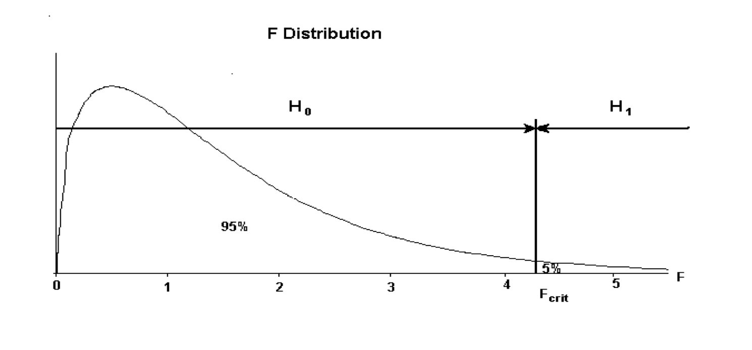
The mechanics of an F-test are as follows:

Two vital pieces of information are required for an F-test: $F_{calc}$ and $F_{crit}$.
$F_{calc}$ is displayed within the R’s standard output. $F_{crit}$ however is a figure derived from degrees of freedom elements and a designated level of significance. For hypothesis testing the $5\%$ significance ($\alpha = 5\%$) level is commonly used. The degrees of freedom elements are
1. Regression: number of explanatory variables in the model
2. Error: number of observations minus the number of estimated $b$ coefficients in the fitted regression model
The all important decision making rule is: if $F_{calc}$ is less than $F_{crit}$ then the null hypothesis $H_0$ is accepted; if $F_{calc}$ is larger than $F_{crit}$ then the alternative hypothesis $H_1$ is accepted:

if $F_{calc} < F_{crit} => H_0$

if $F_{calc} > F_{crit} => H_1$

This formal test involves a rather weak alternative hypothesis, which says only that $R^2$ is significantly bigger than $0$. If $H_1$ is accepted we will have to make a judgement, without the aid of any further formal test, about the usefulness of $R^2$ and hence the model being studied.

$R^2 Adjusted$

$R^2$ can also be used in comparing competing models. If two or more models have been put forward to explain the same response variable then a reasonable rule is to rank the explanatory power of the models in terms of their $R^2$ values. Thus the model with the highest $R^2$ value would be the best model.

The information gathered from the individual regressions carried out in Test a) can be used to give an initial judgement and ranking of the relative importance of the various explanatory variables.

However this rule should be used carefully. It is a valid rule when the competing models have the same number of explanatory variables. It is not valid when comparing models that have different numbers of explanatory variables. It is intuitively obvious that a model with more explanatory variables will have a better chance of explaining the $Y$ variable than a model with fewer variables. Thus the highest $R^2$ rule is biased in favour of those models with more explanatory variables even when some of these explanatory variables are not very useful. In an attempt to redress the imbalance when comparing models with different numbers of explanatory variables, a different version of $R^2$ called $R^2_{adjusted}$ has been developed as follows:

\[\bar{R}^2 = 1 - \frac{(n-1)}{(n-(k+1))}(1-R^2)\]

💡 Note that the mathematically adopted way of writing $R^2_{adjusted}$ is $\bar{R}^2$.

By examining $\bar{R}^2$ it can be seen that when $k$ goes up it is possible for the value of $\bar{R}^2$ to fall. Thus this statistic gives a better way of comparing models with different values for $k$. As before the rule for comparing models is straightforward: choose the model with the highest $\bar{R}^2$.

Test c) t-tests: Individually, are the explanatory variables important?

Using $R^2$ to judge the ‘goodness’ of the set of explanatory variables does not tell us anything about the importance of any one single explanatory variable. Just because a set of variables is important does not necessarily mean that each individual variable is contributing towards explaining the behaviour of $Y$. What is needed is a test than enables us to check the validity of each variable one at a time. Such a test procedure is available as follows:

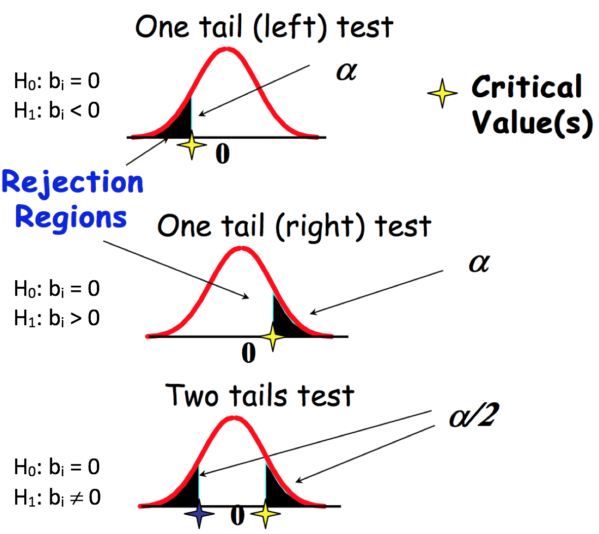
$H_0: b_i = 0$ (explanatory variable $i$ is not important)
$H_1: b_i < 0$ (explanatory variable $i$ has a positive influence) or
- $H_1: b_i > 0$ (explanatory variable $i$ has a negative influence) or
- $H_1: b_i \neq 0$ (explanatory variable $i$ has an influence)

The appropriate $H_1$ for any particular variable is crucially connected with the prior view as to the nature of the connection between any one proposed explanatory variable and the response variable.

The appropriate test statistic involves a t-test based on $(n-(k+1))$ degrees of freedom.

The critical region, denoted by $H_1$, is crucially dependent upon the nature of the alternative hypothesis as put forward by the data analyst. $t_{calc}$ is generated from the R output. $t_{crit}$ is a combination of the Degrees of Freedom from Error and the level of test significance. $t_{crit}$ is the benchmark helping to determine whether one accepts or rejects the null Hypothesis.

If $t_{calc}$ lies in the critical region then the alternative hypothesis is accepted and the modeller accepts that the explanatory variable does have an influence on the behaviour of $Y$. If this is not the case and $t_{calc}$ lies in the $H_0$ area, we will accept that the explanatory variable is useless and that it should be eliminated from the model.

The hypothesis testing methodology typically adopts the $\alpha = 5\%$ level of significance and can be illustrated as follows:

Once all the variables have been individually analysed a further regression command should be given on all remaining acceptable explanatory variables in order to ascertain the best fitted model.

Some of the decision making outcomes from the series of t-test may be uncomfortable in terms of the information from other tests and we may have to experiment with various competing fitted models using subtle combinations of prior views, $R^2$, $\bar{R}^2$ values, and $F$, $t-test$ outcomes before selecting a best model or a set of equally good models.

There are many other, more sophisticated, tests that can be used to judge the validity, i.e. usefulness of a fitted regression model. Before we familiarise ourselves with them and in order to appreciate their practicality and effectiveness, we will conduct an analysis for fitting a multiple regression model based on the procedure explained above.

$p$-Value Approach for Hypothesis Testing

The $p$-value is a probability of obtaining a value of the test statistic or a more extreme value of the test statistic assuming that the null hypothesis is true. Thus, the $p$-value approach involves determining “likely” or “unlikely” by determining the probability, assuming the null hypothesis were true of observing a more extreme test statistic in the direction of the alternative hypothesis than the one observed.

if the $p$-value $\leqslant$ $\alpha$ accept $H_0$ (“unlikely”)
if the $p$-value $\alpha$ reject $H_0$ in favour of $H_1$ (“likely”)

As such, in the context of the inference about the regression parameters, the $p$-values help determine whether the relationships that you observe in your sample also exist in the larger population. The $p$-value for each independent variable tests the null hypothesis that the variable has no effect on the dependent variable. In other words, there is insufficient evidence to conclude that there is effect at the population level.

Case Study

carData::Salaries: The 2008-09 nine-month academic salary for Assistant Professors, Associate Professors and Professors in a college in the U.S. The data was collected as part of the on-going effort of the college’s administration to monitor salary differences between male and female faculty members.

Format: A data frame with 397 observations on the following 6 variables:

rank: a factor with levels:
- AssocProf
- AsstProf
- Prof
discipline: a factor with levels:
- A (“theoretical” departments) or
- B (“applied” departments)
yrs.since.phd: years since PhD
yrs.service: years of service
sex: a factor with levels
- Female
- Male
salary: nine-month salary, in dollars

The first set of questions is:

which of the measured variable is the response variable?
which are the explanatory variables?
are the explanatory variables measured or attribute, or a mixture of both?

Considering that the data is collected for the purpose of the analysis of academic salary we are going to identify salary as the response variable. The rest of the variables we can use as possible factors that can influence the behaviour of the response variable.

The “Standard” regression approach assumes modelling a relationship between measured response and measured explanatory variables. However, often when building multiple regression models we do not want to be limited to the choice of only measured explanatory variables. We also want to be able to include attribute explanatory variables in the multiple regression modelling. In consequence, it is important to learn about supplementary steps that are required to make such models interpretable.

Dummy Variables

As we have learnt previously, attribute variables are vectors of class factor in R. This vector is encoded numerically, with information about the levels of the variable saved in the levels attribute.

# If you don't have carData installed yet, uncomment and run the line below
# install.packages(carData)
library(carData)
data(Salaries)
attach(Salaries)
class(sex)

## [1] "factor"

unclass(sex)

##   [1] 2 2 2 2 2 2 2 2 2 1 2 2 2 2 2 2 2 2 2 1 2 2 2 2 1 2 2 2 2 2 2 2 2 2 1 1 2
##  [38] 2 2 2 2 2 2 2 2 2 2 1 1 2 2 2 1 2 2 2 2 2 2 2 2 2 2 1 2 2 2 2 1 2 2 2 2 2
##  [75] 2 2 2 2 2 2 2 2 2 2 1 2 2 2 2 2 1 2 2 2 2 2 2 2 2 2 2 2 2 1 2 2 2 2 2 2 2
## [112] 2 2 2 1 2 2 2 2 1 2 2 2 1 2 2 2 1 2 2 2 2 1 1 2 2 2 2 2 2 2 2 2 2 2 2 2 2
## [149] 1 2 2 2 2 1 2 2 2 2 2 2 2 2 2 2 2 2 2 2 2 2 2 2 2 2 2 2 2 2 2 1 2 2 2 2 2
## [186] 2 1 2 2 2 2 2 2 2 2 2 2 2 2 2 2 2 2 2 2 2 2 2 2 2 2 2 2 2 2 2 2 2 1 2 2 2
## [223] 2 2 2 2 2 2 2 2 1 1 2 1 2 2 2 1 2 2 2 2 2 2 2 1 2 2 2 2 2 2 2 1 1 2 2 2 2
## [260] 2 2 2 2 2 2 2 2 2 2 2 2 2 2 2 1 2 2 2 2 2 2 2 2 2 2 2 2 2 2 2 2 2 2 2 2 2
## [297] 2 2 2 2 2 2 2 2 2 2 2 2 2 2 2 2 2 2 2 2 1 2 2 2 2 2 2 1 2 2 2 2 2 2 2 2 1
## [334] 2 1 2 2 2 2 2 2 1 2 2 2 2 2 2 2 2 2 2 2 2 2 2 2 2 1 2 2 1 2 2 2 2 2 2 2 2
## [371] 2 2 2 2 2 2 2 2 2 2 2 2 2 2 2 2 2 2 2 2 2 2 2 2 2 2 2
## attr(,"levels")
## [1] "Female" "Male"

Note, that the unclass() function removes the attributes of the sex variable above and prints it using default print method, allowing for easier examination of the internal structure of the object.

However, when using an attribute variable in a linear regression model it would make no sense to treat it as a measured explanatory variable because of its numeric levels. In the context of linear modelling we need to code them to represent the levels of the attribute.

Two-level attribute variables are very easy to code. We simply create an indicator or dummy variable that takes on two possible dummy numerical values. Consider the sex indicator variable. We can code this using a dummy variable $d$: \[\begin{equation} d=\left\{ \begin{array}{@{}ll@{}} 0, & \text{if female} \\ 1, & \text{if male} \end{array}\right. \end{equation}\]

💡 This is the default coding used in R. Zero value is assigned to the level which is first alphabetically, unless it is changed by using the releveld() function for example, or by specifying the levels of the factor variable specifically.

For a simple regression model of salary versus sex:

\[salary = b_0 + b_1sex + e,\]

this results in the model

\[\begin{equation} salary_i = b_0 + b_1sex_i + e_i=\left\{ \begin{array}{@{}ll@{}} b_0 + b_1 \times 1 + e_i = b_0 + b_1 + e_i, & \text{if the person is male} \\ b_0 + b_1 \times 0 + e_i = b_0 + e_i, & \text{if the person is female} \end{array}\right. \end{equation}\]

where $b_0$ can be interpreted as the average $\text{salary}$ for females, and $b_0 + b_1$ as the average $\text{salary}$ for males. The value of $b_1$ represents the average difference in $\text{salary}$ between females and males.

We can conclude that dealing with an attribute variable with two levels in a linear model is straightforward. In this case, a dummy variable indicates whether an observation has a particular characteristic: yes/no. We can observe it as a “switch” in a model, as this dummy variable can only assume the values 0 and 1, where 0 indicates the absence of the effect, and 1 indicates the presence. The values 0/1 can be seen as off/on.

The way in which R codes dummy variables is controlled by the contrast option:

options("contrasts")

## $contrasts
##         unordered           ordered 
## "contr.treatment"      "contr.poly"

The output points out the conversion of the factor into an appropriate set of contrasts. In particular, the first one: for unordered factors, and the second one: the ordered factors. The former one is applicable in our context.

To explicitly identify the coding of the factor, i.e. dummy variable used by R, we can use the contrasts() function.

contrasts(sex)

##        Male
## Female    0
## Male      1

contrasts(discipline)

##   B
## A 0
## B 1

contrasts(rank)

##           AssocProf Prof
## AsstProf          0    0
## AssocProf         1    0
## Prof              0    1

Note that applied “contr.treatment” conversion takes only the value 0 or 1 and that for an attribute variable with k levels it will create k-1 dummy variables. One can argue that the printout of the function could have been more informative by putting indexed letter d as a header for each of the printed columns. For example:

attribute variable sex, where k=2

attribute	$d$
Female	0
Male	1

attribute variable rank, where k=3

attribute	$d_1$	$d_2$
AsstProf	0	0
AssocProf	1	0
Prof	0	1

There are many different ways of coding attribute variables besides the dummy variable approach explained here. All of these different approaches lead to equivalent model fits. What differ are the coefficients, i.e. model parameters as they require different interpretations, arranged to measure particular contrasts. This 0/1 coding implemented in R’s default contr.treatment contrast offers straightforward interpretation of the associated parameter in the model, which often is not the case when implementing other contrasts.

Interpreting coefficients of attribute variables

In the case of measured predictors, we are comfortable with the interpretation of the linear model coefficient as a slope, which tells us what a unit increase in the response variable is, i.e. outcome per unit increase in the explanatory variable. This is not necessarily the right interpretation for attribute explanatory variables.

# average salary values for each sex group
suppressPackageStartupMessages(library(dplyr))
Salaries %>% 
    select(salary, sex) %>%   
    group_by(sex) %>% 
    summarise(mean=mean(salary))

## # A tibble: 2 x 2
##   sex       mean
##   <fct>    <dbl>
## 1 Female 101002.
## 2 Male   115090.

If we obtain the mean salary for each sex group we will find that for female professors the average salary is $\$101,002$ and for male professors the average is $\$115,090$. That is, a difference of $\$14,088$. If we now look at the parameters of the regression model for salary vs sex where females are coded as zero and males as one, we get exactly the same information, implying that the coefficient is the estimated difference in average between the two groups.

# regression model 
lm(salary ~  sex)

## 
## Call:
## lm(formula = salary ~ sex)
## 
## Coefficients:
## (Intercept)      sexMale  
##      101002        14088

For more on this topic check the following link: Categorical variables and interaction terms in linear regression

Fitting a Multivariate Regression Model

We are interested in the extent to which variation in the response variable salary is associated with variation in the explanatory variables available in the Salaries data set, that is we want to fit a multiple linear regression model to the given data. The model we wish to construct should contain enough to explain relations in the data and at the same time be simple enough to understand, explain to others, and use.

For convenience we will adopt the following notation:

$y$: salary
$x_1$: yrs.since.phd
$x_2$: yrs.service
$x_3$: discipline
$x_4$: sex
$x_5$: rank

Generally, in multiple regression we have a continuous response variable and two or more continuous explanatory variables, however in this dataset we have three attribute variables that we wish to include as the explanatory variables in the model.

Next, we need to specify the model that embodies our mechanistic understanding of the factors involved and the way that they are related to the response variable. It would make sense to expect that all of the available $x$ variables may impact the behaviour of $y$, thus the model we wish to build should reflect our viewpoint, i.e. $y = f(x_1, x_2, x_3, x_4, x_5)$:

\[y = b_0 + b_1x_1 + b_2x_2 + b_3x_3 + b_4x_4 + b_5x_5 + e\] Our viewpoint states a belief that all explanatory variables have positive impact on the response. For example, more years in service will cause higher salary.

Our objective now is to determine the values of the parameters in the model that lead to the best fit of the model to the data. That is, we are not only trying to estimate the parameters of the model, but we are also seeking the minimal adequate model to describe the data.

The best model is the model that produces the least unexplained variation following the principle of parsimony rather than complexity. That is the model should have as few parameters as possible, subject to the constraint that the parameters in the model should all be statistically significant.

For regression modelling in R we use the lm() function, that fits a linear model assuming normal errors and constant variance. We specify the model by a formula that uses arithmetic operators: +, -, *, / and ^ which enable different functionalities from their ordinary ones. But, before we dive into statistical modelling of the given data, we need to take a first step and conduct the most fundamental task of data analysis procedure: Get to Know Our Data.

Examining multivariate data is intrinsically more challenging than examining univariate and bivariate data. To get the most in-depth vision into multivariate data behaviour we construct scatter plot matrices that enable the display of pairwise relationships. In R, the scatter plot matrices are composed by the pairs() function, which comes as a part of the default graphics package. Since we wish to include attribute variables in our analysis we are going to use the GGally::ggpairs() function that produces a pairwise comparison of multivariate data for both data types: measured and attribute.

# If you don't have GGally installed yet, uncomment and run the line below
# install.packages(GGally)
suppressPackageStartupMessages(library(GGally))
ggpairs(Salaries)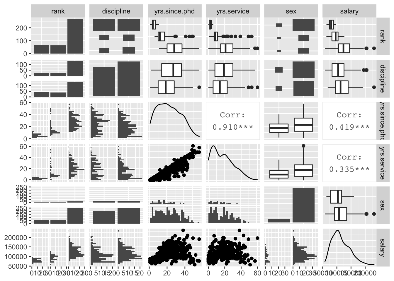

This is an information rich visualisation that includes pairwise relationships of all the variables we want to consider for our model. By focusing on the last column of the plots, we can notice influence from all explanatory variables onto the response, except maybe for discipline and sex. We also notice unbalanced representation of the groups for variables rank and sex, but for the purpose of our practice in fitting a multi factor model this isn’t too problematic. We need to be especially concerned with the extent of correlations between the explanatory variables and what is of particular interest to us is the high multicollinearity between rank, yrs.since.phd and yrs.service, which happens when the variables are highly linearly related. As a consequence, we will need to keep an eye on the significance of using all of these variables in the model.

Fitting the Model

There are no fixed rules when fitting the linear models, but there are adopted standards that have proven to work well in practice. We start off by fitting a maximal model then we carry on simplifying it by removing non-significant explanatory variables. This needs to be done with caution, making sure that the simplifications make good scientific sense, and do not lead to significant reductions in explanatory power. Although this should be the adopted strategy for fitting a model it is not a guarantee to finding all the important structures in a complex data frame.

We can summarise our model building procedure algorithm as follows:

Fit the maximal model that includes all the variables
- Assess the overall significance of the model by checking how big the $R^2$/$\bar{R}^2$ is. If statistically significant, carry on with the model fitting procedure, otherwise stop (F-test)
Remove the least significant terms one at a time
- Check variables’ $t_{calculated}$ values and perform a one tail or two tail t-test depending on your prior view
- If the deletion causes an insignificant increase in $\bar{R}^{2}$ leave that term out of the model
Keep removing terms from the model until the model contains nothing but significant terms.

# model_1 <- lm(salary ~ yrs.since.phd + yrs.service + discipline + sex + rank, data = Salaries) #long handed way
model_1 <- lm(salary ~ ., data = Salaries) # full stop, . , implies: all other variables in data that do not already appear in the formula
summary(model_1)

## 
## Call:
## lm(formula = salary ~ ., data = Salaries)
## 
## Residuals:
##    Min     1Q Median     3Q    Max 
## -65248 -13211  -1775  10384  99592 
## 
## Coefficients:
##               Estimate Std. Error t value Pr(>|t|)    
## (Intercept)    65955.2     4588.6  14.374  < 2e-16 ***
## rankAssocProf  12907.6     4145.3   3.114  0.00198 ** 
## rankProf       45066.0     4237.5  10.635  < 2e-16 ***
## disciplineB    14417.6     2342.9   6.154 1.88e-09 ***
## yrs.since.phd    535.1      241.0   2.220  0.02698 *  
## yrs.service     -489.5      211.9  -2.310  0.02143 *  
## sexMale         4783.5     3858.7   1.240  0.21584    
## ---
## Signif. codes:  0 '***' 0.001 '**' 0.01 '*' 0.05 '.' 0.1 ' ' 1
## 
## Residual standard error: 22540 on 390 degrees of freedom
## Multiple R-squared:  0.4547, Adjusted R-squared:  0.4463 
## F-statistic:  54.2 on 6 and 390 DF,  p-value: < 2.2e-16

Overall, is the model a good fit? How big is the $R^2$/$\bar{R}^2$?

The $R^2 = 45.47\%$ and the $\bar{R}^2 = 44.63\%$ are well above the value of zero allowing us to accept this as a valid model without having to formally test it to assess its statistical significance. It manages to explain almost half of the variability in the response variable salary.

Individually, are the explanatory variables important?

We identify the sex explanatory variable as clearly not significant, which is in line with the conclusion we could draw from the boxplot in the pairwise comparison plot for salary vs. sex. We will remove it to begin the process of model simplification.

#model_1 <- lm(salary ~ yrs.since.phd + yrs.service + discipline + sex + rank, data = Salaries) # long handed method
model_2 <- update(model_1,~. - sex) # refitting by removing the least significant term
summary(model_2)

## 
## Call:
## lm(formula = salary ~ rank + discipline + yrs.since.phd + yrs.service, 
##     data = Salaries)
## 
## Residuals:
##    Min     1Q Median     3Q    Max 
## -65244 -13498  -1455   9638  99682 
## 
## Coefficients:
##               Estimate Std. Error t value Pr(>|t|)    
## (Intercept)    69869.0     3332.1  20.968  < 2e-16 ***
## rankAssocProf  12831.5     4147.7   3.094  0.00212 ** 
## rankProf       45287.7     4236.7  10.689  < 2e-16 ***
## disciplineB    14505.2     2343.4   6.190 1.52e-09 ***
## yrs.since.phd    534.6      241.2   2.217  0.02720 *  
## yrs.service     -476.7      211.8  -2.250  0.02497 *  
## ---
## Signif. codes:  0 '***' 0.001 '**' 0.01 '*' 0.05 '.' 0.1 ' ' 1
## 
## Residual standard error: 22550 on 391 degrees of freedom
## Multiple R-squared:  0.4525, Adjusted R-squared:  0.4455 
## F-statistic: 64.64 on 5 and 391 DF,  p-value: < 2.2e-16

We note a slight reduction in $\bar{R^2}$ from $44.63\%$ to $44.55\%$ which we can regard as an insignificant decrease. The next step is to check the coefficients and assess for the effect of the remaining variables. We identify yrs.since.phd and yrs.service as the least influential in explaining the variability of salary. To illustrate how to formally assess their effect, we will conduct the t-test for the yrs.since.phd variable:

$H_0: b_{ysp} = 0$
$H_1: b_{ysp} > 0$

=========================

If $t_{calc} < t_{crit} => H_0$
If $t_{calc} > t_{crit} => H_1$

qt(0.95, 391)

## [1] 1.64876

As $t_{calc} = 2.217 > t_{crit} = 1.64876 => H_1$ we will keep the remaining variable and stop with the model simplification and focus on its interpretation.

We can take a closer look at the coefficients of our fitted model:

coef(model_2)

##   (Intercept) rankAssocProf      rankProf   disciplineB yrs.since.phd 
##    69869.0110    12831.5375    45287.6890    14505.1514      534.6313 
##   yrs.service 
##     -476.7179

The structure of our final fitted model is:

\[y = b_0 + b_1x_1 + b_2x_2 + b_3x_3 + b_4x_4 + e,\] where

$y$: salary
$x_1$: yrs.since.phd
$x_2$: yrs.service
$x_3$: discipline
$x_4$: rank

We can take a closer look at the coefficients of our fitted model:

coef(model_2)

##   (Intercept) rankAssocProf      rankProf   disciplineB yrs.since.phd 
##    69869.0110    12831.5375    45287.6890    14505.1514      534.6313 
##   yrs.service 
##     -476.7179

Examining the output we realise that R has created three “sub” dummy variables for the variable rank: \[ dr_1 = \begin{cases} 1 & \text{rank is AsstProf} \\ 0 & \text{for rank is not AsstProf} \end{cases} \]

\[ dr_2 = \begin{cases} 1 & \text{rank is AssocProf} \\ 0 & \text{rank is not AssocProf} \end{cases} \]

\[ dr_3 = \begin{cases} 1 & \text{rank is Prof} \\ 0 & \text{rank is not Prof} \end{cases} \]

It has chosen to use the model: \[ y = b_0 + b_1dr_2 + b_2dr_3 + b_3d_1 + b_4x_1 + b_5x_2 + e, \]

where:

$y$ is salary
$x_1$ is yrs.since.phd
$x_2$ is yrs.service
$dr_2$ and $dr_3$ are the dummy variables defined above for the purpose of coding variable rank
$d_1$ is a dummy variable used in the coding of variable discipline as explained earlier

Note that R doesn’t need to use $dr_1$, to create three models; it only needs two dummy variables since it is using $dr_1$ as a reference level, also known as the base line. This subsequently allows R to create three models relating to rank variable:

AsstProf: $y = b_0 + b_3d_1 + b_4x_1 + b_5x_2 + e$
AssocProf: $y = (b_0 + b_1) + b_3d_1 + b_4x_1 + b_5x_2 + e$
Prof: $y = (b_0 + b_2) + b_3d_1 + b_4x_1 + b_5x_2 + e$

telling us that:

$b_0$ is average salary for Assistant Professor who works in a “theoretical” department and $b_0 + b_3$ average salary for Assistant Professor who works in an “applied” department
$(b_0 + b_1)$ is average salary for Associate Professor who works in a “theoretical” department and $(b_0 + b_1) + b_3$ average salary for Associate Professor who works in an “applied” department
$(b_0 + b_2)$ is average salary for Professor who works in a “theoretical” department and $(b_0 + b_2) + b_3$ average salary for Professor who works in an “applied” department

Learning this we can make an interpretation of our final fitted model as follows:

For every year since PhD (yrs.since.phd) on average salary (salary) will go up by $\$534.63$ assuming the rest of the variables are fixed in the model
For every year in service (yrs.service) on average salary (salary) will go down by $\$476.72$ assuming the rest of the variables are fixed in the model
Average salary of an Assistant Professor (rank: AsstProf) who works in a “theoretical” department is $\$69,869.01$ and who works in an “applied” department is $\$84,374.16$; this can vary for the number of years in service and since PhD
Average salary of an Associate Professor (rank: AssocProf) who works in a “theoretical” department is $\$82,700.55$ and who works in an “applied” department is $\$97,205.70$; this can vary for the number of years in service and since PhD
Average salary of a Professor (rank: Prof) who works in a “theoretical” department is $\$115,156.70$ and who works in an “applied” department is $\$129,661.90$; this can vary for the number of years in service and since PhD

This model explains around $45\%$ of the variability in the response variable salary.

Adding ~ 0 to lm() formula enables R to suppress the intercept. Note that if we remove the intercept, then we can directly obtain all “three intercepts” without a base level to fit the final fitted model:

model_2_1 <- lm(salary ~  0 + rank + discipline + yrs.since.phd + yrs.service)
summary(model_2_1)

## 
## Call:
## lm(formula = salary ~ 0 + rank + discipline + yrs.since.phd + 
##     yrs.service)
## 
## Residuals:
##    Min     1Q Median     3Q    Max 
## -65244 -13498  -1455   9638  99682 
## 
## Coefficients:
##               Estimate Std. Error t value Pr(>|t|)    
## rankAsstProf   69869.0     3332.1  20.968  < 2e-16 ***
## rankAssocProf  82700.5     3916.7  21.115  < 2e-16 ***
## rankProf      115156.7     4350.9  26.467  < 2e-16 ***
## disciplineB    14505.2     2343.4   6.190 1.52e-09 ***
## yrs.since.phd    534.6      241.2   2.217   0.0272 *  
## yrs.service     -476.7      211.8  -2.250   0.0250 *  
## ---
## Signif. codes:  0 '***' 0.001 '**' 0.01 '*' 0.05 '.' 0.1 ' ' 1
## 
## Residual standard error: 22550 on 391 degrees of freedom
## Multiple R-squared:  0.9638, Adjusted R-squared:  0.9633 
## F-statistic:  1736 on 6 and 391 DF,  p-value: < 2.2e-16

Adding a Complexity

So far we have seen that by fitting an additive regression model to the data, we aim to identify and understand how the value of a dependent response variable changes when any one of the independent explanatory variables is changed while the other independent variables stay the same. This is a restrictive form of a model as it only allows for linear relationships between the response and the explanatory variables, and the way in which one explanatory variable affects the response is the same for any value of the other explanatory variables used in the model.

We need to add flexibility to accommodate these limitations. This will allow the use of linear models for non-linear relationships and in which the effect of one explanatory variable can be different for different values of the other explanatory variable by introducing the concept of interaction. This brings more complexity into the multivariate regression model.

Case Study: The Quality of red Bordeaux Vintages

To illustrate the multivariate model fitting procedure with interactions we are going to use wine.csv available from Eduardo García Portugués’s book: Notes for Predictive Modeling. The dataset is formed by the auction Price of 27 red Bordeaux vintages, five vintage descriptors (WinterRain, AGST, HarvestRain, Age, Year), and the population of France in the year of the vintage, FrancePop.

Year: year in which grapes were harvested to make wine
Price: logarithm of the average market price for Bordeaux vintages according to 1990–1991 auctions. The price is relative to the price of the 1961 vintage, regarded as the best one ever recorded
WinterRain: winter rainfall (in mm)
AGST: Average Growing Season Temperature (in degrees Celsius)
HarvestRain: harvest rainfall (in mm)
Age: age of the wine measured as the number of years stored in a cask
FrancePop: population of France at Year (in thousands)

We would like to analyse the quality of a vintage that has been quantified as the price and make the interpretation of our statistical findings.

Don’t forget!!! 🤔 First things first: Get to Know Data 🤓

We will start this analysis by examining the pairwise plot.

wine = read.csv("https://raw.githubusercontent.com/egarpor/handy/master/datasets/wine.csv")
summary(wine)

##       Year          Price         WinterRain         AGST        HarvestRain   
##  Min.   :1952   Min.   :6.205   Min.   :376.0   Min.   :14.98   Min.   : 38.0  
##  1st Qu.:1960   1st Qu.:6.508   1st Qu.:543.5   1st Qu.:16.15   1st Qu.: 88.0  
##  Median :1967   Median :6.984   Median :600.0   Median :16.42   Median :123.0  
##  Mean   :1967   Mean   :7.042   Mean   :608.4   Mean   :16.48   Mean   :144.8  
##  3rd Qu.:1974   3rd Qu.:7.441   3rd Qu.:705.5   3rd Qu.:17.01   3rd Qu.:185.5  
##  Max.   :1980   Max.   :8.494   Max.   :830.0   Max.   :17.65   Max.   :292.0  
##       Age          FrancePop    
##  Min.   : 3.00   Min.   :43184  
##  1st Qu.: 9.50   1st Qu.:46856  
##  Median :16.00   Median :50650  
##  Mean   :16.19   Mean   :50085  
##  3rd Qu.:22.50   3rd Qu.:53511  
##  Max.   :31.00   Max.   :55110

ggpairs(wine)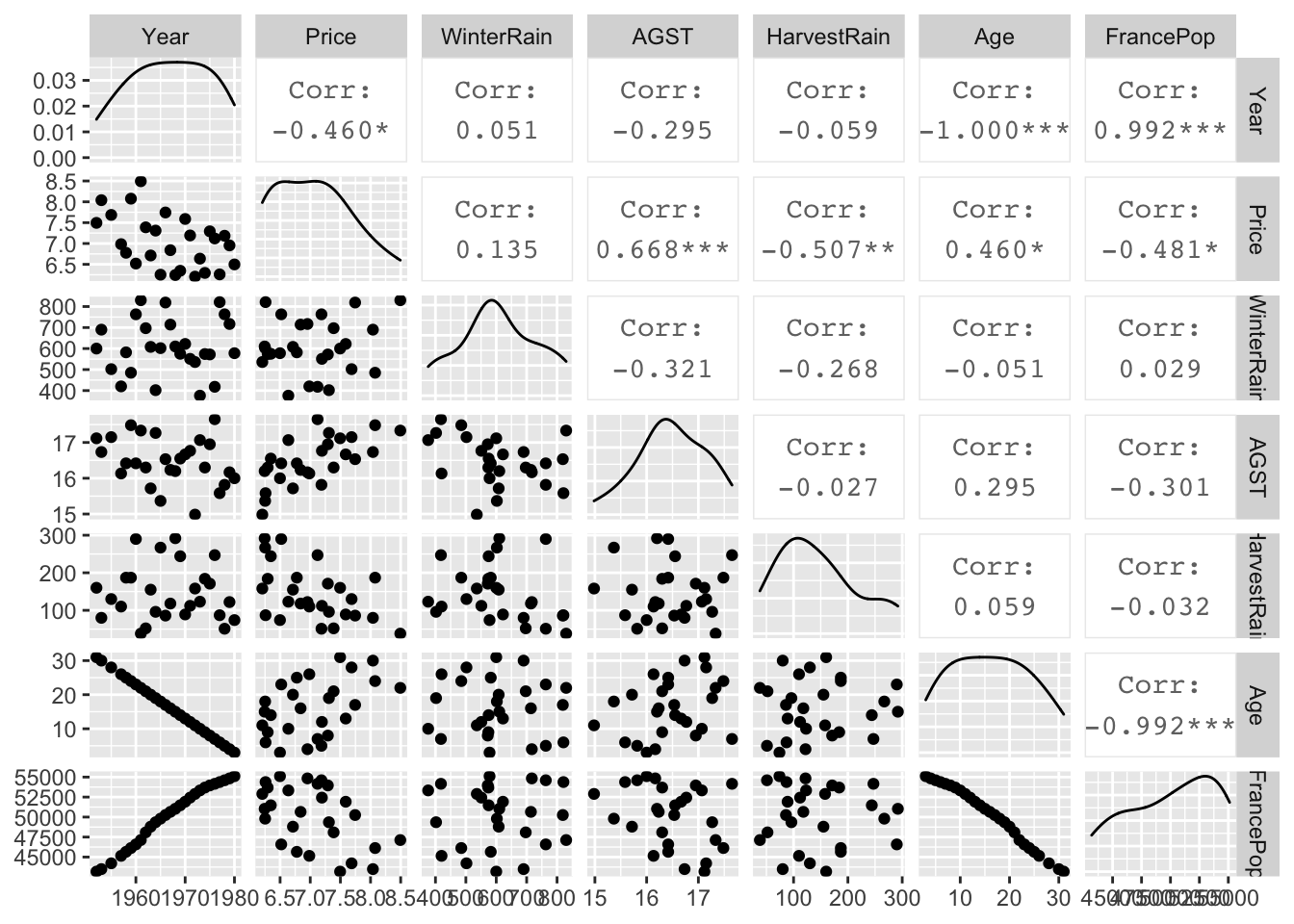

What conclusions can we draw:

We can notice a perfect relationship between the variables Year and Age. This is to be expected since this data was collected in 1983 and Age was calculated as: Age = 1983 - Year. Knowing this, we are going to remove Year from the analysis and use Age as it will be easier to interpret.
There is a strong relationship between Year, ie. Age and FrancePop and since we want to impose our viewpoint that the total population does not influence the quality of wine we will not consider this variable in the model.
We are going to investigate possible interactions between the rainfall (WinterRain) and growing season temperature (AGST). In R this will be created automatically by using the * operator.

Let us build a model:

We will start with the most complicated model that includes the highest-order interaction.

In R we will specify the three-way interaction, which will automatically add all combinations of two-way interactions.

model1 <- lm(Price ~ WinterRain + AGST + HarvestRain + Age + WinterRain * AGST * HarvestRain, data = wine)
summary(model1)

## 
## Call:
## lm(formula = Price ~ WinterRain + AGST + HarvestRain + Age + 
##     WinterRain * AGST * HarvestRain, data = wine)
## 
## Residuals:
##      Min       1Q   Median       3Q      Max 
## -0.35058 -0.19462 -0.02645  0.17194  0.52079 
## 
## Coefficients:
##                               Estimate Std. Error t value Pr(>|t|)   
## (Intercept)                  8.582e+00  1.924e+01   0.446   0.6609   
## WinterRain                  -1.858e-02  2.896e-02  -0.642   0.5292   
## AGST                        -1.748e-01  1.137e+00  -0.154   0.8795   
## HarvestRain                 -4.713e-02  1.540e-01  -0.306   0.7631   
## Age                          2.476e-02  8.288e-03   2.987   0.0079 **
## WinterRain:AGST              1.272e-03  1.712e-03   0.743   0.4671   
## WinterRain:HarvestRain       7.836e-05  2.600e-04   0.301   0.7665   
## AGST:HarvestRain             3.059e-03  9.079e-03   0.337   0.7401   
## WinterRain:AGST:HarvestRain -5.446e-06  1.540e-05  -0.354   0.7278   
## ---
## Signif. codes:  0 '***' 0.001 '**' 0.01 '*' 0.05 '.' 0.1 ' ' 1
## 
## Residual standard error: 0.2833 on 18 degrees of freedom
## Multiple R-squared:  0.8621, Adjusted R-squared:  0.8007 
## F-statistic: 14.06 on 8 and 18 DF,  p-value: 2.675e-06

The model explains well over $80\%$ of variability and is clearly a strong model, but the key question is whether we can simplify it. We will start the process of this model simplification by removing the three-way interaction as it is clearly not significant.

model2 <- update(model1, ~. -WinterRain:AGST:HarvestRain, data =wine)
summary(model2)

## 
## Call:
## lm(formula = Price ~ WinterRain + AGST + HarvestRain + Age + 
##     WinterRain:AGST + WinterRain:HarvestRain + AGST:HarvestRain, 
##     data = wine)
## 
## Residuals:
##      Min       1Q   Median       3Q      Max 
## -0.35245 -0.19452  0.01643  0.17289  0.51420 
## 
## Coefficients:
##                          Estimate Std. Error t value Pr(>|t|)   
## (Intercept)             2.980e+00  1.066e+01   0.279  0.78293   
## WinterRain             -9.699e-03  1.408e-02  -0.689  0.49930   
## AGST                    1.542e-01  6.383e-01   0.242  0.81168   
## HarvestRain             6.496e-03  2.610e-02   0.249  0.80610   
## Age                     2.441e-02  8.037e-03   3.037  0.00678 **
## WinterRain:AGST         7.490e-04  8.420e-04   0.890  0.38484   
## WinterRain:HarvestRain -1.350e-05  7.338e-06  -1.840  0.08144 . 
## AGST:HarvestRain       -1.032e-04  1.520e-03  -0.068  0.94656   
## ---
## Signif. codes:  0 '***' 0.001 '**' 0.01 '*' 0.05 '.' 0.1 ' ' 1
## 
## Residual standard error: 0.2767 on 19 degrees of freedom
## Multiple R-squared:  0.8611, Adjusted R-squared:  0.8099 
## F-statistic: 16.83 on 7 and 19 DF,  p-value: 6.523e-07

The $\bar{R}^2$ has slightly increased in value. Next, we remove the least significant two-way interaction term.

model3 <- update(model2, ~. -AGST:HarvestRain, data = wine)
summary(model3)

## 
## Call:
## lm(formula = Price ~ WinterRain + AGST + HarvestRain + Age + 
##     WinterRain:AGST + WinterRain:HarvestRain, data = wine)
## 
## Residuals:
##      Min       1Q   Median       3Q      Max 
## -0.35424 -0.19343  0.01176  0.17161  0.51218 
## 
## Coefficients:
##                          Estimate Std. Error t value Pr(>|t|)   
## (Intercept)             3.518e+00  6.946e+00   0.507  0.61802   
## WinterRain             -1.017e-02  1.195e-02  -0.851  0.40488   
## AGST                    1.218e-01  4.138e-01   0.294  0.77147   
## HarvestRain             4.752e-03  4.553e-03   1.044  0.30901   
## Age                     2.451e-02  7.710e-03   3.179  0.00472 **
## WinterRain:AGST         7.769e-04  7.166e-04   1.084  0.29119   
## WinterRain:HarvestRain -1.342e-05  7.059e-06  -1.902  0.07174 . 
## ---
## Signif. codes:  0 '***' 0.001 '**' 0.01 '*' 0.05 '.' 0.1 ' ' 1
## 
## Residual standard error: 0.2697 on 20 degrees of freedom
## Multiple R-squared:  0.8611, Adjusted R-squared:  0.8194 
## F-statistic: 20.66 on 6 and 20 DF,  p-value: 1.35e-07

Again, it is reassuring to notice an increase in the $\bar{R}^2$, but we can still simplify the model further by removing another least significant two-way interaction term.

model4 <- update(model3, ~. -WinterRain:AGST, data = wine)
summary(model4)

## 
## Call:
## lm(formula = Price ~ WinterRain + AGST + HarvestRain + Age + 
##     WinterRain:HarvestRain, data = wine)
## 
## Residuals:
##     Min      1Q  Median      3Q     Max 
## -0.5032 -0.1934  0.0109  0.1771  0.4621 
## 
## Coefficients:
##                          Estimate Std. Error t value Pr(>|t|)    
## (Intercept)            -3.812e+00  1.598e+00  -2.386 0.026553 *  
## WinterRain              2.747e-03  9.471e-04   2.900 0.008560 ** 
## AGST                    5.586e-01  9.495e-02   5.883 7.71e-06 ***
## HarvestRain             4.717e-03  4.572e-03   1.032 0.313877    
## Age                     2.785e-02  7.094e-03   3.926 0.000774 ***
## WinterRain:HarvestRain -1.349e-05  7.088e-06  -1.903 0.070835 .  
## ---
## Signif. codes:  0 '***' 0.001 '**' 0.01 '*' 0.05 '.' 0.1 ' ' 1
## 
## Residual standard error: 0.2708 on 21 degrees of freedom
## Multiple R-squared:  0.8529, Adjusted R-squared:  0.8179 
## F-statistic: 24.35 on 5 and 21 DF,  p-value: 4.438e-08

There is an insignificant decrease in $\bar{R}^2$. We notice HarvestRain is now the least significant term, but it is used for the WinterRain:HarvestRain interaction, which is significant at $\alpha = 5\%$ and therefore we should keep it. However, as the concept of parsimony prefers a model without interactions to a model containing interactions between variables, we will remove the remaining interaction term and see if it significantly affects the explanatory power of the model.

model5 <- update(model4, ~. -WinterRain:HarvestRain, data = wine)
summary(model5)

## 
## Call:
## lm(formula = Price ~ WinterRain + AGST + HarvestRain + Age, data = wine)
## 
## Residuals:
##      Min       1Q   Median       3Q      Max 
## -0.46024 -0.23862  0.01347  0.18601  0.53443 
## 
## Coefficients:
##               Estimate Std. Error t value Pr(>|t|)    
## (Intercept) -3.6515703  1.6880876  -2.163  0.04167 *  
## WinterRain   0.0011667  0.0004820   2.420  0.02421 *  
## AGST         0.6163916  0.0951747   6.476 1.63e-06 ***
## HarvestRain -0.0038606  0.0008075  -4.781 8.97e-05 ***
## Age          0.0238480  0.0071667   3.328  0.00305 ** 
## ---
## Signif. codes:  0 '***' 0.001 '**' 0.01 '*' 0.05 '.' 0.1 ' ' 1
## 
## Residual standard error: 0.2865 on 22 degrees of freedom
## Multiple R-squared:  0.8275, Adjusted R-squared:  0.7962 
## F-statistic: 26.39 on 4 and 22 DF,  p-value: 4.057e-08

The $\bar{R}^2$ is reduced by around $2\%$, but it has all the significant terms and it is easier to interpret. For those reasons and in the spirit of parsimony that argues that a model should be as simple as possible, we can suggest that this should be regarded as the best final fitted model.

We realise that for the large numbers of explanatory variables, and many interactions and non-linear terms, the process of model simplification can take a very long time. There are many algorithms for automatic variable selection that can help us to chose the variables to include in a regression model. Stepwise regression and Best Subsets regression are two of the more common variable selection methods.

The stepwise procedure starts from the saturated model (or the maximal model, whichever is appropriate) through a series of simplifications to the minimal adequate model. This progression is made on the basis of deletion tests: F tests, AIC, t-tests or chi-squared tests that assess the significance of the increase in deviance that results when a given term is removed from the current model.

The best subset regression (BREG), also known as “all possible regressions”, as the name of the procedure indicates, fits a separate least squares regression for each possible combination of the $p$ predictors, i.e. explanatory variables. After fitting all of the models, BREG then displays the best fitted models with one explanatory variable, two explanatory variables, three explanatory variables, and so on. Usually, either adjusted R-squared or Mallows Cp is the criterion for picking the best fitting models for this process. The result is a display of the best fitted models of different sizes up to the full/maximal model and the final fitted model can be selected by comparing displayed models based on the criteria of parsimony.

“These methods are frequently are abused by naive researchers who seek to interpret the order of entry of variables into the regression equation as an index of their ‘‘importance.’’ This practice is potentially misleading.” J. Fox and S. Weisberg book: An R Companion to Applied Regression, Third Edition, Sage (2019)

💡 When selecting a model one should remember the important concept of parsimony!

As M.J. Crawley points out in his well know editions of “The R Book” we need to remember that models are portrayals of phenomena that should be both “accurate and convenient” and the principle of parsimony is an essential tool for model exploration. As he suggests: “just because we go to the trouble of measuring something does not mean we have to have it in our model.”

"Parsimony says that, other things being equal, we prefer:

a model with $n−1$ parameters to a model with n parameters
a model with $k−1$ explanatory variables to a model with k explanatory variables
a linear model to a model which is curved
a model without a hump to a model with a hump
a model without interactions to a model containing interactions between factors" Crawley, M.J. 2013, The R Book. 2nd Edition. John Wiley, New York

Useful links:

Summary

For problems ranging from bioinformatics to marketing, many analysts prefer to develop “classifiers” instead of developing predictive models

Further Reading

Claeskens, G. and Hjort, N.L. (2008) Model Selection and Model Averaging, Cambridge University Press, Cambridge.

Fox, J. (2002) An R and S-Plus Companion to Applied Regression, Sage, Thousand Oaks, CA.

YOUR TURN 👇

Go back to the Salaries data Case Study:

Adding ~0 to lm() formula enables R to suppress the intercept. Try to fit the following model by removing the intercept.

model_2_1 <- lm(salary ~  0 + rank + discipline + yrs.since.phd + yrs.service)
summary(model_2_1)

This will allow you to obtain all “three intercepts” without a reference level.

Does this model differ from the previously fitted model_2? Provide justified explanation
Interpret the model

Can the final fitted model developed for the Salaries data Case Study be further simplified? Justify your answer

Use Prestige data available from the carData package of datasets designed to accompany J. Fox and S. Weisberg book: An R Companion to Applied Regression, Third Edition, Sage (2019). Fit a multivariate model that explains variation in the response variable prestige, explaining the reasons behind the steps taken with appropriate interpretation of the final fitted model.

carData::Prestige: The Canadian occupational prestige data, where the observations are occupations. Justification for treating the 102 occupations as a sample implicitly rests on the claim that they are “typical” of the population, at least with respect to the relationship between prestige and income.

education: Average education of occupational incumbents, years, in 1971.
income: Average income of incumbents, dollars, in 1971.
women: Percentage of incumbents who are women.
prestige: Pineo-Porter prestige score for occupation, from a social survey conducted in the mid-1960s.
census: Canadian Census occupational code.
type: Type of occupation. A factor with levels (note: out of order):
- bc: Blue Collar
- prof: Professional, Managerial, and Technical
- wc: White Collar

The dataset Prostate available in the package lasso2 contains information on 97 men who were about to receive a radical prostatectomy. This data set comes from a study examining the correlation between the prostate specific antigen (lpsa) and a number of other clinical measures.

Select the best subset model to predict lpsa using all the available predictors.

Take a look at vignette for the lasso2 package