Clasification
Classification is a form of supervised learning focused on building and evaluating models for qualitative response, which we often refer to as categorical response. For example, is someone a smoker is a qualitative variable taking values yes and no. Another example would be European Country, which is a qualitative variable taking qualitative values: Italy, France, Spain, Great Britain, Germany, Serbia,… Here, we will study approaches for predicting qualitative responses, a process that is known as classification.
Predicting a qualitative response for an observation can be referred to as classifying that observation, since it assigns to a category, or class. Classification methods tend to predict the probability of each of the categories of a qualitative variable as a basis for generating the classification. In this sense they also behave like regression methods. Although many of the regression modelling techniques can be used for classification, the way we evaluate model performance is, needless to say, different since MSE and \(R^2\) are not appropriate in the context of classification.
Classification problems occur often, perhaps even more so than regression problems. Classification methods have wide practical applications. In environmental studies they are used to assess flood susceptibility. They are a popular financial tool for the assessment of bankruptcy prediction. In medical studies, breast cancer is often classified according to the number of oestrogen receptors present on the tumour. These are just a few of many examples where classification methods are used to perform the prediction.
There are many classification methods, also known as classifiers, that can be used to predict a qualitative response. We will familiarise ourself with the two most widely-used classifiers: K-nearest neighbours and logistic regression.
K-nearest neighbours
K-nearest neighbours (KNN) algorithm is one of the simplest techniques used in machine learning. Because of its simplicity and low calculation time KNN is a popular classification method preferred by many. It is a simple recommendation system used by Amazon and Netflix (see Use of KNN for the Netflix Prize). It is a non-parametric method meaning that the model is made up entirely from the data given to it, instead of being based on the assumptions about the structure of the given data. In other words the KNN approach makes no assumptions about the shape of the decision boundary.
When implementing KNN, the first step is to transform data points into feature vectors, or their mathematical value. The algorithm then works by finding the distance between the mathematical values of these points. The most common way to find this distance is the Euclidean distance
\[ \begin{equation} \begin{split} d(p, q) & = d(q, p) \\ & & = \sqrt{(p_1 - q_1)^2 + (p_2 - q_2)^2 + \dotsc + (p_n - q_n)^2} \\ & &= \sqrt{\sum_{i=1}^{n}(p_i-q_i)^2} \end{split} \end{equation} \] where
- \(p\) and \(q\) are two points in Euclidean \(n\)-space and
- \(q_i\) and \(p_i\) are Euclidean vectors, starting from the origin of the space (initial point).
This can be illustrated as

The figure below provides an illustrative example of the KNN approach. It consists of a small training data set of twelve red dots and twelve green squares. The goal is to make a prediction for the point labelled by the yellow star. For the choice of \(K=3\) the KNN will identify the three observations that are closest to the yellow star. These neighbour observations are shaded in the circle around the yellow star. It consists of two red points and one green square, resulting in estimated probabilities of 2/3 for the red circle class and 1/3 for the green square class. As a result KNN will predict that the yellow star belongs to the red circle class.

Let us assume we are dealing with a problem of classification of animals into two categories: dogs or cats. Classification needs to be conducted in respect of the two measurements:
- Measurement A: The length of the animal (in cm) from the tip of its nose to the back of its body, excluding the tail
- Measurement B: The height of the animal’s leg from floor to shoulder (in cm)
We have a test data with the length and height measurements of several dogs and cats. For a new set of observed measurements we need to be able to determine if they belong to a dog or a cat. That is, the unknown animal needs to be classified into one of the two groups based on the given measurements. To do this we create a 2D plane like the one above. Next, we follow the same procedure of calculating the distance of the new object from the older ones, and the closer it is to either one of the categories will determine its own category.
animal <- as.factor(c("cat", "dog", "cat", "cat", "dog", "dog", "dog", "cat", "cat", "dog", "cat", "dog", "unknown"))
A <- c(40, 34, 43, 37, 30, 39, 40, 43, 42, 37, 41, 35, 39)
B <- c(24, 20, 23, 21, 26, 30, 39, 25, 27, 35, 18, 28, 20)

animals_data <- data.frame(animal, A, B)

library(ggplot2)
ggplot(animals_data, aes(x = A, y = B)) +
  geom_point(aes(col = animal), shape = 20, size = 3) +
  geom_point(x = 39, y = 20, shape = 13, size = 7) +
  labs (title= "Cat & Dogs",
        x = "length", y = "height") +
  theme_minimal() +
  theme(legend.position = "bottom",
        panel.border = element_rect(fill = NA,
                                    colour = "black",
                                    size = .75),
        plot.title=element_text(hjust=0.5)) +
scale_colour_brewer(palette = "Set1") 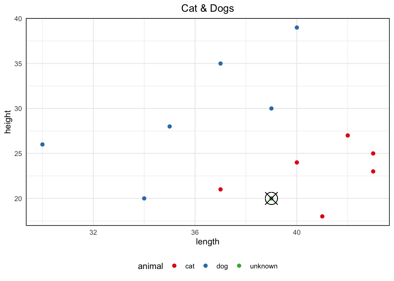
We can see that the new animal with 20cm of height and 39cm of length is in proximity with cats more than dogs. Hence, we predict that the new animal is a cat. However, in most cases we will deal with situations in which categories will be defined by many more attributes that will prevent us from simply drawing them on a scatter diagram like we did in this example.
The more arguments describing the categories we have greater chance of appropriate prediction there is. For example if we get two more measurements to consider:
- Measurement C: The width of the animal (in cm) across the shoulders, or the widest part of the animal if not the shoulders
- Measurement D: The height of the animal (in cm) from the ground to the top of its head, including the ears if they are erect
we simply use the above stated Euclidean formula to calculate the distance of the new upcoming animal from the already given animals. We take the square root of
\[\sqrt{(A_1-A_2)^2 + (B_1-B_2)^2 + (C_1-C_2)^2 + (D_1-D_2)^2}\]
where 1 is representing the already drawn data point and 2 is representing the new data point that you want to determine the category of. This calculation shown above will be used with every data point available. That is, it will run as many times as there are rows in your dataset.
KNN summary
When running the KNN algorithm we first need to define the value \(K\). If \(K\) is 3 it will check the 3 closest neighbours in order to determine the category. If the majority of neighbours belong to a certain category from within those three nearest neighbours, then that will be chosen as the category of the upcoming object.
As different variables have different scaling units, like weight in kg and height in cm, they need to be normalised prior to their use in the calculation of their distance:
\[\text{standardised } x =\frac{(x-min(x))}{(min(x) — max(x))}\] This will convert the values onto a scale 0 to 1.
Note that this can be done with numerical variables, which is not to say that KNN cannot deal with categorical variables too. There is much more than just Euclidean distance that can be used in the KNN algorithm. There are various theoretical measures which may be much more appropriate in those cases: Jaccard similarity, Tanimoto coefficient, Sørensen–Dice coefficient and so on.
In a nutshell, when running the KNN algorithm, data should be normalised prior to splitting it into training and testing sets. KNN runs a formula to compute the distance between each data point and the test data. It then finds the probability of these points being similar to the test data and classifies it based on which points share the highest probabilities.
Example in R
When calculating distances between data points in the KNN algorithm, we must use numeric predictor variables only. However, the outcome variable for KNN classification should remain a factor variable.
In the following examples we will apply the KNN classification in R using two packages: the class and the caret. We will also conduct KNN classification on two data sets: one in which all predictor variables are the measured type and the other data set in which some of the predictor variables are attribute variables with a different number of levels.
Using the class package and the iris data
To run the KNN algorithm in R we will use the knn() function which is part of the class package. This function requires the following input information:
- a matrix containing the predictor associated with the training data:
training.X - a matrix containing the predictor associated with the data for which we wish to make predictors:
test.X - a vector containing the class labels for the training observations:
train - a number of nearest neighbours to be used by the classifier:
K
Let us illustrate the K Nearest Neighbours algorithm classification on the well known Iris Dataset. This famous (Fisher’s or Anderson’s) iris data set gives the measurements in centimetres of the variables’ sepal length and width and petal length and width, respectively, for 50 flowers from each of 3 species of iris. The species are Iris setosa, versicolor, and virginica.
# load iris data
suppressPackageStartupMessages(library(dplyr))
data("iris")
glimpse(iris)
## Rows: 150
## Columns: 5
## $ Sepal.Length <dbl> 5.1, 4.9, 4.7, 4.6, 5.0, 5.4, 4.6, 5.0, 4.4, 4.9, 5.4, 4.…
## $ Sepal.Width <dbl> 3.5, 3.0, 3.2, 3.1, 3.6, 3.9, 3.4, 3.4, 2.9, 3.1, 3.7, 3.…
## $ Petal.Length <dbl> 1.4, 1.4, 1.3, 1.5, 1.4, 1.7, 1.4, 1.5, 1.4, 1.5, 1.5, 1.…
## $ Petal.Width <dbl> 0.2, 0.2, 0.2, 0.2, 0.2, 0.4, 0.3, 0.2, 0.2, 0.1, 0.2, 0.…
## $ Species <fct> setosa, setosa, setosa, setosa, setosa, setosa, setosa, s…Note that apart from the Species category the rest of the variables are all numeric types.
Since classification is a type of Supervised Learning, we will would require two sets of data: training data and test data. Hence, we will divide the dataset into two subsets in the proportions of 80:20 percent. Since the iris dataset is sorted by Species by default, we will first have to mix up the data rows and then take the subset:
iris.train: training subsetiris.test: testing subset
set.seed(123) # required to reproduce the results
rnums<- sample(rep(1:150)) # randomly generate numbers from 1 to 150; 150 - number of rows
iris<- iris[rnums, ] # jumbling up "iris" dataset by randomising
#head(iris, n=10)
DT::datatable(iris)
Remember that data should be normalised prior to splitting it into training and testing sets. Therefore, as our next step we will normalise data, scaling it to a z-score metric to have values between 0 and 1, after which we will split it into two subsets: training and testing.
# normalise data
normalise <- function(x){
  return ((x-min(x)) / (max(x)-min(x)))
}

iris_norm <- as.data.frame(lapply(iris[,c(1,2,3,4)], normalise))
#head(iris_norm, n=10)
DT::datatable(iris_norm)
# split data
iris_train <- iris_norm[1:120, ]
iris_train_target <- iris[1:120, 5]
iris_test <- iris_norm[121:150, ]
iris_test_target <- iris[121:150, 5]
summary(iris_norm)## Sepal.Length Sepal.Width Petal.Length Petal.Width
## Min. :0.0000 Min. :0.0000 Min. :0.0000 Min. :0.00000
## 1st Qu.:0.2222 1st Qu.:0.3333 1st Qu.:0.1017 1st Qu.:0.08333
## Median :0.4167 Median :0.4167 Median :0.5678 Median :0.50000
## Mean :0.4287 Mean :0.4406 Mean :0.4675 Mean :0.45806
## 3rd Qu.:0.5833 3rd Qu.:0.5417 3rd Qu.:0.6949 3rd Qu.:0.70833
## Max. :1.0000 Max. :1.0000 Max. :1.0000 Max. :1.00000Once we have prepared our data for the application of the KNN classification we can run the algorithm. We can also obtain predicted probabilities, given test predictors by setting the probability argument as true: prob = TRUE.
# If you don't have class installed yet, uncomment and run the line below
#install.packages("class")
library(class)
model_knn <- knn(train = iris_train,
                 test = iris_test,
                 cl = iris_train_target,
                 k = 10,
                 prob  = TRUE)
model_knn
## [1] versicolor versicolor setosa virginica versicolor virginica
## [7] setosa setosa versicolor virginica versicolor setosa
## [13] versicolor versicolor setosa versicolor versicolor versicolor
## [19] versicolor setosa versicolor virginica setosa setosa
## [25] setosa setosa versicolor virginica versicolor virginica
## attr(,"prob")
##  [1] 1.0 0.9 1.0 0.7 1.0 1.0 1.0 1.0 0.7 1.0 1.0 1.0 0.9 1.0 1.0 1.0 1.0 0.8 0.9
## [20] 1.0 1.0 1.0 1.0 1.0 1.0 1.0 0.9 1.0 1.0 1.0
## Levels: setosa versicolor virginicaattributes(model_knn)$prob## [1] 1.0 0.9 1.0 0.7 1.0 1.0 1.0 1.0 0.7 1.0 1.0 1.0 0.9 1.0 1.0 1.0 1.0 0.8 0.9
## [20] 1.0 1.0 1.0 1.0 1.0 1.0 1.0 0.9 1.0 1.0 1.0Unfortunately, this only returns the predicted probability of the most common class. In the binary case, this would be sufficient to recover all probabilities, however, for multi-class problems, we cannot recover each of the probabilities of interest. This will simply be a minor annoyance for now, which we will fix when we introduce the caret package for model training.
A common method for describing the performance of a classification model is the confusion matrix. So, to check how well the model has performed we will construct the confusion matrix, which is a table that is used to show the number of correct and incorrect predictions on a classification problem when the real values of the test data are known. For a two class problem it is of the format

The TRUE values are the number of correct predictions made.
how_well <- data.frame(model_knn, iris_test_target) %>%
  mutate(result = model_knn == iris_test_target)

how_well
## model_knn iris_test_target result
## 1 versicolor versicolor TRUE
## 2 versicolor versicolor TRUE
## 3 setosa setosa TRUE
## 4 virginica versicolor FALSE
## 5 versicolor versicolor TRUE
## 6 virginica virginica TRUE
## 7 setosa setosa TRUE
## 8 setosa setosa TRUE
## 9 versicolor versicolor TRUE
## 10 virginica virginica TRUE
## 11 versicolor versicolor TRUE
## 12 setosa setosa TRUE
## 13 versicolor versicolor TRUE
## 14 versicolor versicolor TRUE
## 15 setosa setosa TRUE
## 16 versicolor versicolor TRUE
## 17 versicolor versicolor TRUE
## 18 versicolor versicolor TRUE
## 19 versicolor versicolor TRUE
## 20 setosa setosa TRUE
## 21 versicolor versicolor TRUE
## 22 virginica virginica TRUE
## 23 setosa setosa TRUE
## 24 setosa setosa TRUE
## 25 setosa setosa TRUE
## 26 setosa setosa TRUE
## 27 versicolor versicolor TRUE
## 28 virginica virginica TRUE
## 29 versicolor versicolor TRUE
## 30 virginica virginica TRUEconfusion_matrix <- table(iris_test_target, model_knn)
summary(model_knn)## setosa versicolor virginica
## 10 14 6confusion_matrix## model_knn
## iris_test_target setosa versicolor virginica
## setosa 10 0 0
## versicolor 0 14 1
## virginica 0 0 5The values on the diagonal shows the number of correctly classified instances for each category. In our example it is showing that the KNN algorithm has correctly classified 29 instances out of a total 30 data points in the test data. The values not on the diagonal imply that they have been incorrectly classified. In our case it is only 1 observation, giving an accuracy of 97%.
The simplest metric for model classification is the overall accuracy rate. To evaluate predicted classes, we are going to create a function that can calculate the accuracy of the KNN algorithm.
# calculate percentage accuracy
accuracy <- function(x){
  sum(diag(x) / (sum(rowSums(x)))) * 100
}
accuracy(confusion_matrix)
## [1] 96.66667Although the overall accuracy rate might be easy to compute and to interpret, it makes no distinction about the type of errors being made. Choosing the correct level of flexibility is critical to the success of any machine learning method. For the KNN method this can be adjusted by trying different values of K, but the bias-variance trade off can make this a difficult task.
Using the caret package and the penguins data
The R’s caret package (classification and regression training) holds many functions that help to build predictive models. It holds tools for data splitting, pre-processing, feature selection, tuning and supervised – unsupervised learning algorithms, etc. The caret package provides direct access to various functions for training a model with a machine learning algorithm for KNN classification. But, before we can use caret to perform various tasks to carry out the necessary machine learning work, we need to familiarise ourselves with our data.
The penguins data set is available from the palmerpenguins package. It includes 6 measurements of 344 penguin species and information about the year during which data was collected. We will start by loading the R packages we will need for this exercise and reading the penguins data set.
# If you don't have tidyr, caret, gmodels, psych, palmerpenguins and pscl installed yet, uncomment and run the lines below
#install.packages("tidyr")
#install.packages("caret")
#install.packages("gmodels")
#install.packages("psych")
#install.packages("palmerpenguins")
#install.packages("pscl") # pR2()
suppressPackageStartupMessages(library(dplyr))
suppressPackageStartupMessages(library(tidyr))
suppressPackageStartupMessages(library(caret))
suppressPackageStartupMessages(library(gmodels)) # CrossTable()
suppressPackageStartupMessages(library(psych)) # dummy.code()
library(palmerpenguins)
library(ggplot2)

penguins <- read.csv(path_to_file("penguins.csv"))
glimpse(penguins)
## Rows: 344
## Columns: 8
## $ species <chr> "Adelie", "Adelie", "Adelie", "Adelie", "Adelie", "A…
## $ island <chr> "Torgersen", "Torgersen", "Torgersen", "Torgersen", …
## $ bill_length_mm <dbl> 39.1, 39.5, 40.3, NA, 36.7, 39.3, 38.9, 39.2, 34.1, …
## $ bill_depth_mm <dbl> 18.7, 17.4, 18.0, NA, 19.3, 20.6, 17.8, 19.6, 18.1, …
## $ flipper_length_mm <int> 181, 186, 195, NA, 193, 190, 181, 195, 193, 190, 186…
## $ body_mass_g <int> 3750, 3800, 3250, NA, 3450, 3650, 3625, 4675, 3475, …
## $ sex <chr> "male", "female", "female", NA, "female", "male", "f…
## $ year <int> 2007, 2007, 2007, 2007, 2007, 2007, 2007, 2007, 2007…speciesa factor denoting penguin species (Adélie, Chinstrap and Gentoo)islanda factor denoting an island in the Palmer Archipelago, Antarctica (Biscoe, Dream or Torgersen)bill_length_mma number denoting bill length (millimetres)bill_depth_mma number denoting bill depth (millimetres)flipper_length_mman integer denoting flipper length (millimetres)body_mass_gan integer denoting body mass (grams)sexa factor denoting penguin sex (female, male)yearan integer denoting the study year (2007, 2008 or 2009)
For k-NN classification, we are going to predict the categorical variable species using all the other variables within the data set. This data set has both measured and attribute variables as the predictors. As year is a variable of the recording we will not consider it in our modelling and therefore we will remove it from the data set we will work with. ML algorithms are sensitive to missing values. For the aim of this analysis, instead of constructing imputation for the missing values we will simply drop them from the data set.
pingo <- penguins[1:7]

pingo %>%
  summarise_all(funs(sum(is.na(.)))) %>%
  pivot_longer(cols = 1:7, names_to = 'columns', values_to = 'NA_count') %>%
  arrange(desc(NA_count)) %>%
  ggplot(aes(y = columns, x = NA_count)) + geom_col(fill = 'deepskyblue4') +
  geom_label(aes(label = NA_count)) +
  theme_minimal() +
  labs(title = 'Penguins - NA Count',
       caption = "Visualisation: https://www.r-bloggers.com/2020/06/penguins-dataset-overview-iris-alternative-in-r",
       y = "variables") +
  theme(plot.title = element_text(hjust = 0.5))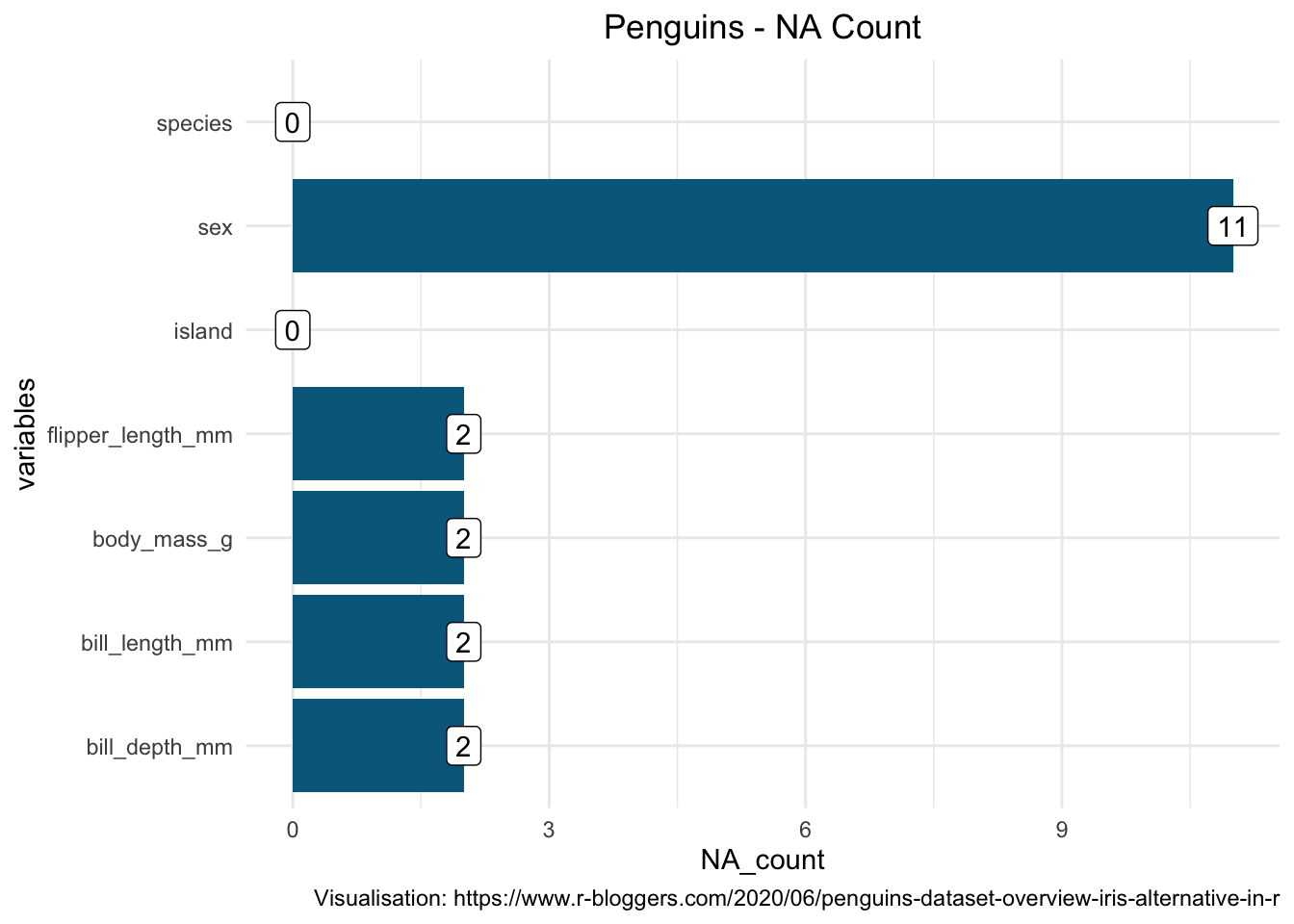
data_class <- pingo %>%
  drop_na()
Next, we need to prepare data further for our k-NN classification. First, we will put our outcome variable species into its own object and remove it from the data set.
species_outcome <- data_class %>% select(species)

# remove original variable from the data set
data_class <- data_class %>% select(-species)

glimpse(data_class)
## Rows: 333
## Columns: 6
## $ island <chr> "Torgersen", "Torgersen", "Torgersen", "Torgersen", …
## $ bill_length_mm <dbl> 39.1, 39.5, 40.3, 36.7, 39.3, 38.9, 39.2, 41.1, 38.6…
## $ bill_depth_mm <dbl> 18.7, 17.4, 18.0, 19.3, 20.6, 17.8, 19.6, 17.6, 21.2…
## $ flipper_length_mm <int> 181, 186, 195, 193, 190, 181, 195, 182, 191, 198, 18…
## $ body_mass_g <int> 3750, 3800, 3250, 3450, 3650, 3625, 4675, 3200, 3800…
## $ sex <chr> "male", "female", "female", "female", "male", "femal…We see that bill_length_mm, bill_depth_mm, flipper_length_mm and body_mass_g are measured variables of which the features are measured on different metrics, which means they have to be scaled. To do this we are going to use the scale function, which means we are scaling to a z-score metric.
data_class[, c("bill_length_mm",
               "bill_depth_mm",
               "flipper_length_mm",
               "body_mass_g")] <- scale(data_class[, c("bill_length_mm",
                                                      "bill_depth_mm",
                                                      "flipper_length_mm",
                                                      "body_mass_g")])
glimpse(data_class)
## Rows: 333
## Columns: 6
## $ island <chr> "Torgersen", "Torgersen", "Torgersen", "Torgersen", …
## $ bill_length_mm <dbl> -0.8946955, -0.8215515, -0.6752636, -1.3335592, -0.8…
## $ bill_depth_mm <dbl> 0.77955895, 0.11940428, 0.42409105, 1.08424573, 1.74…
## $ flipper_length_mm <dbl> -1.4246077, -1.0678666, -0.4257325, -0.5684290, -0.7…
## $ body_mass_g <dbl> -0.567620576, -0.505525421, -1.188572125, -0.9401915…
## $ sex <chr> "male", "female", "female", "female", "male", "femal…head(data_class)## island bill_length_mm bill_depth_mm flipper_length_mm body_mass_g sex
## 1 Torgersen -0.8946955 0.7795590 -1.4246077 -0.5676206 male
## 2 Torgersen -0.8215515 0.1194043 -1.0678666 -0.5055254 female
## 3 Torgersen -0.6752636 0.4240910 -0.4257325 -1.1885721 female
## 4 Torgersen -1.3335592 1.0842457 -0.5684290 -0.9401915 female
## 5 Torgersen -0.8581235 1.7444004 -0.7824736 -0.6918109 male
## 6 Torgersen -0.9312674 0.3225288 -1.4246077 -0.7228585 femaleAs our next step in preparing data for the application of the KNN algorithm we need to dummy code attribute variables. From data description we know that the variable island is an attribute variable that has three levels and sex is an attribute variable with two levels.
We will first dummy code the attribute variable sex that has only two levels and then the one with more than two levels using the dummy.code() function from the psych package.
data_class$sex <- dummy.code(data_class$sex)For island, the variable dummy.code() function will create three new variables coded with 0 and 1, which will then need to be combined with the original data set. As the final preparation, since we have created a single variable for each island category we will now remove the original island variable from our data.
island <- as.data.frame(dummy.code(data_class$island))
data_class <- cbind(data_class, island)
data_class <- data_class %>% select(-island)

glimpse(data_class)
## Rows: 333
## Columns: 8
## $ bill_length_mm <dbl> -0.8946955, -0.8215515, -0.6752636, -1.3335592, -0.8…
## $ bill_depth_mm <dbl> 0.77955895, 0.11940428, 0.42409105, 1.08424573, 1.74…
## $ flipper_length_mm <dbl> -1.4246077, -1.0678666, -0.4257325, -0.5684290, -0.7…
## $ body_mass_g <dbl> -0.567620576, -0.505525421, -1.188572125, -0.9401915…
## $ sex <dbl[,2]> <matrix[26 x 2]>
## $ Biscoe <dbl> 0, 0, 0, 0, 0, 0, 0, 0, 0, 0, 0, 0, 0, 0, 0, 1, …
## $ Dream <dbl> 0, 0, 0, 0, 0, 0, 0, 0, 0, 0, 0, 0, 0, 0, 0, 0, 0, 0…
## $ Torgersen <dbl> 1, 1, 1, 1, 1, 1, 1, 1, 1, 1, 1, 1, 1, 1, 1, 0, 0, 0…print.data.frame(head(data_class, ))## bill_length_mm bill_depth_mm flipper_length_mm body_mass_g sex.male
## 1 -0.8946955 0.7795590 -1.4246077 -0.5676206 1
## 2 -0.8215515 0.1194043 -1.0678666 -0.5055254 0
## 3 -0.6752636 0.4240910 -0.4257325 -1.1885721 0
## 4 -1.3335592 1.0842457 -0.5684290 -0.9401915 0
## 5 -0.8581235 1.7444004 -0.7824736 -0.6918109 1
## 6 -0.9312674 0.3225288 -1.4246077 -0.7228585 0
## sex.female Biscoe Dream Torgersen
## 1 0 0 0 1
## 2 1 0 0 1
## 3 1 0 0 1
## 4 1 0 0 1
## 5 0 0 0 1
## 6 1 0 0 1Once we have prepared data, we can run the KNN algorithm. First, we will split the data into training and test sets. We partition 80% of the data into the training set and the remaining 20% into the test set.
set.seed(1) # set the seed to make the partition reproducible

# 80% of the sample size
smp_size <- floor(0.80 * nrow(data_class))

train_ind <- sample(seq_len(nrow(data_class)), size = smp_size)

# creating test and training sets that contain all of the predictors
class_pred_train <- data_class[train_ind, ]
class_pred_test <- data_class[-train_ind, ]
We will also split the response variable into training and test sets using the same partition as above.
species_outcome_train <- species_outcome[train_ind, ]
species_outcome_test <- species_outcome[-train_ind, ]
We will start by using the knn() classification function available from the class package. There are several rules of thumb we can use when choosing the number of k. One that we will adopt is the square root of the number of observations in the training set, which in our case is 266. So, in this case, we select 16 as the number of neighbours.
pingo_knn <- knn(train = class_pred_train, test = class_pred_test, cl = species_outcome_train, k=16)


# put "species_outcome_test" in a data frame
species_outcome_test <- data.frame(species_outcome_test)

# merge "pingo_knn" and "species_outcome_test"
class_comparison <- data.frame(pingo_knn, species_outcome_test)

# specify column names for "class_comparison"
names(class_comparison) <- c("predicted_species", "observed_species")

# inspect "class_comparison"
DT::datatable(class_comparison)
To evaluate the model, this time we will construct the confusion matrix by using the CrossTable() function available from the gmodels package.
CrossTable(x = class_comparison$observed_species, y = class_comparison$predicted_species, prop.chisq=FALSE, prop.c = FALSE, prop.r = FALSE, prop.t = FALSE)##
##
## Cell Contents
## |-------------------------|
## | N |
## |-------------------------|
##
##
## Total Observations in Table: 67
##
##
## | class_comparison$predicted_species
## class_comparison$observed_species | Adelie | Chinstrap | Gentoo | Row Total |
## ----------------------------------|-----------|-----------|-----------|-----------|
## Adelie | 31 | 0 | 0 | 31 |
## ----------------------------------|-----------|-----------|-----------|-----------|
## Chinstrap | 1 | 10 | 0 | 11 |
## ----------------------------------|-----------|-----------|-----------|-----------|
## Gentoo | 0 | 0 | 25 | 25 |
## ----------------------------------|-----------|-----------|-----------|-----------|
## Column Total | 32 | 10 | 25 | 67 |
## ----------------------------------|-----------|-----------|-----------|-----------|
##
## The results of the confusion matrix indicate that our model predicts species very well. The numbers are all zeros in the off-diagonals apart from one case in which a penguin from the Chinstrap class has been classified as Adelie. This is indicating that our model has successfully classified the outcome based on the given predictors.
Next, we will run the KNN classification using the caret package which ‘authomatically’ picks the optimal number of neighbours K.
### caret

pingo_knn_caret <- train(class_pred_train,
                         species_outcome_train,
                         method = "knn",
                         preProcess = c("center", "scale"))

pingo_knn_caret
## k-Nearest Neighbors
##
## 266 samples
## 8 predictor
## 3 classes: 'Adelie', 'Chinstrap', 'Gentoo'
##
## Pre-processing: centered (7), scaled (7), ignore (1)
## Resampling: Bootstrapped (25 reps)
## Summary of sample sizes: 266, 266, 266, 266, 266, 266, ...
## Resampling results across tuning parameters:
##
## k Accuracy Kappa
## 5 0.9904743 0.9849471
## 7 0.9934275 0.9897027
## 9 0.9930282 0.9890629
##
## Accuracy was used to select the optimal model using the largest value.
## The final value used for the model was k = 7.Looking at the output of the caret package KNN model, we can see that it chose K = 7, given that this was the number at which accuracy and kappa peaked. Kappa statistic is a measure of inter-rater reliability which is a more robust measure than a simple percent agreement calculation. However, its interpretation is not as intuitive and easy to comprehend as a single percentage measure. For more on the kappa statistic see the Statistic How To website.
plot(pingo_knn_caret)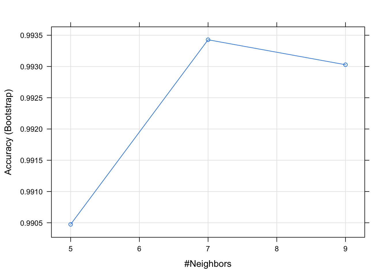
Next, we compare our predicted values of species to our actual values. We also print the confusion matrix, which will give an indication of how well our model has predicted the actual values. In the caret package the confusion matrix output also shows overall model statistics and statistics by class.
We can see that we have obtained the same results as previously. Do you have any suggestions why that may be?
knn_predict <- predict(pingo_knn_caret, newdata = class_pred_test)

confusionMatrix(knn_predict, as.factor(species_outcome_test$species_outcome_test))
## Confusion Matrix and Statistics
##
## Reference
## Prediction Adelie Chinstrap Gentoo
## Adelie 31 1 0
## Chinstrap 0 10 0
## Gentoo 0 0 25
##
## Overall Statistics
##
## Accuracy : 0.9851
## 95% CI : (0.9196, 0.9996)
## No Information Rate : 0.4627
## P-Value [Acc > NIR] : < 2.2e-16
##
## Kappa : 0.9757
##
## Mcnemar's Test P-Value : NA
##
## Statistics by Class:
##
## Class: Adelie Class: Chinstrap Class: Gentoo
## Sensitivity 1.0000 0.9091 1.0000
## Specificity 0.9722 1.0000 1.0000
## Pos Pred Value 0.9688 1.0000 1.0000
## Neg Pred Value 1.0000 0.9825 1.0000
## Prevalence 0.4627 0.1642 0.3731
## Detection Rate 0.4627 0.1493 0.3731
## Detection Prevalence 0.4776 0.1493 0.3731
## Balanced Accuracy 0.9861 0.9545 1.0000So far we have learnt how to prepare data for KNN as well as conduct k-NN classification. In the next section we will learn about another popular classification method: logistic regression.
Logistic Regression
Often in studies, we encounter outcomes that are not continuous, but instead fall into 1 of 2 categories. In these cases we have binary outcomes, variables that can have only two possible values:
- Measuring a performance labeled as \(Y\). Candidates are classified as “good” or “poor”, coded as 1 and 0 respectively, i.e. \(Y\)=1 representing good performance and \(Y\)=0 representing poor performance.
- Risk factor for cancer: person has cancer (\(Y\)=1), or does not (\(Y\)=0)
- Whether a political candidate is going to win an election: lose \(Y\)=0, win \(Y\)=1
- ‘Health’ of a business can be observed by monitoring the solvency of the firm: bankrupt \(Y\)=0, solvent \(Y\)=1
Here \(Y\) is the binary response variable, that is coded as 0 or 1 and rather than predicting these two values for binary response we try to model the probabilities that \(Y\) takes one of these two values.
Let us examine one such example using the bankruptcies data available from 👉 https://tanjakec.github.io/mydata/Bankruptcies.csv.
Bankruptcies.csv file contains data of the operating financial ratios of 66 firms which either went bankrupt or remained solvent after a 2 years period. The data is taken from the book “Regression Analysis by Example” by Chatterjee and Hadi. The variables are:
- three financial ratios (the explanatory variables; measured variables):
- \(X_1\): Retained Earnings / Total Assets
- \(X_2\): Earnings Before Interest and Taxes / Total Assets
- \(X_3\): Sales / Total Assets
- a binary response variable \(Y\):
- 0 - if bankrupt after 2 years
- 1 - if solvent after 2 years
bankrup <- read.csv("https://tanjakec.github.io/mydata/Bankruptcies.csv")
summary(bankrup)
## Y X1 X2 X3
## Min. :0.0 Min. :-308.90 Min. :-280.000 Min. :0.100
## 1st Qu.:0.0 1st Qu.: -39.05 1st Qu.: -17.675 1st Qu.:1.025
## Median :0.5 Median : 7.85 Median : 4.100 Median :1.550
## Mean :0.5 Mean : -13.63 Mean : -8.226 Mean :1.721
## 3rd Qu.:1.0 3rd Qu.: 35.75 3rd Qu.: 14.400 3rd Qu.:1.975
## Max. :1.0 Max. : 68.60 Max. : 34.100 Max. :6.700Since
- linear regression expects a numeric response variable and
- we are interested in the analysis of the risk, ie. the probability of a firm going bankrupt based on its Retained Earnings / Total Assets ratio (RE/TA ratio) figure
it would be very attractive to be able to use the same modelling techniques as for linear models. We are going to do just that: fit a simple linear regression model to examine this relationship to see if it will work.
\[Y = b_0 + b_1X_3\]
model_lm = lm(Y ~  X1, data = bankrup)
# plot a scatter diagram of Y vs X1
plot(Y ~  X1, data = bankrup,
     col = "orangered", pch = "|", ylim = c(-0.2, 1.2),
     main = "using linear regression function for binomial Y")
abline(h = 0, lty = 3)
abline(h = 1, lty = 3)
abline(h = 0.5, lty = 2)
abline(model_lm, lwd = 3, col = "navy")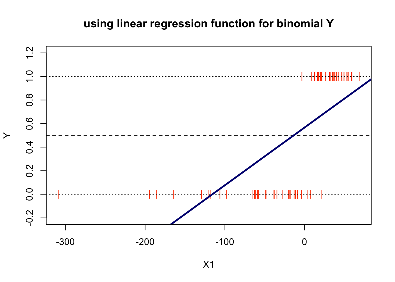
Examining this plot we can make two obvious observations:
the higher the ration of RE/TA the better the chances is for the firm to be solvent
by analysing the risk we analyse a chance, a probability of a company being solvent based on the value of the RE/TA. Since \(Y\) is limited to the values of 0 and 1, rather than predicting these two values we will try to model the probabilities \(p\) that \(Y\) takes one of these two values.
Let \(p\) denote the probability that \(Y\) = 1 when \(X = x\). If we use the standard linear model to describe \(p\), then our model for the probability would be
\[p = P(Y = 1 | X = x) = b_0 + b_1x + e\]
Note that since \(p\) is a probability it must lie between 0 and 1. It seems rational that \(X\hat{b}\) is a reasonable estimate of \(P(Y=1∣X=x)\). Nonetheless, the plot has flagged a big issue with this model and that is that it has predicted probabilities less than 0.
As we can see the linear regression model does not work for this type of problem, for which we do not expect predictions that are off-scale values: below zero or above 1.
Apart from the fact that the linear function given is unbounded, and hence cannot be used to model probability, the other assumptions of linear regression when dealing with this type of a problem are also not valid:
- the relationship between \(Y\) and \(X\) is nonlinear
- error terms are not normally distributed
- the assumption of equal/constant variance (homoscedasticity) dos not hold
A workaround these issues is to fit a different model, one that is bounded by the minimum and maximum probabilities. It makes better sense to model the probabilities on a transformed scale and this is what is done in logistic regression analysis. The relationship between the probability \(p\) and \(X\) can be presented by a logistic regression function.

The shape of the S-curve given in the figure above can be reproduced if we model the probabilities as follows
\[p = P(Y = 1 | X = x) = \frac{e^{\beta_0 + \beta_1x}}{1 + e^{\beta_0 + \beta_1x}},\]
where \(e\) is the base of the natural logarithm. The logistic model can be generalized directly to the situation where we have several predictor variables. The probability \(p\) is modelled as
\[p = P(Y = 1 | X_1 = x_1, X_2=x_2, ..., X_q=x_q) = \frac{e^{\beta_0 + \beta_1x_1 + \beta_2x_2 + ... + \beta_qx_q}}{1 + e^{\beta_0 + \beta_1x_1 + \beta_2x_2 + ... + \beta_qx_q}},\] where \(q\) is the number of predictors. The two equations above are called the logistic regression functions. It is nonlinear in the parameters \(\beta_0, \beta_1,... \beta_q\). However, it can be linearised by the logit transformation. Instead of working directly with \(p\) we work with a transformed value of \(p\). If \(p\) is the probability of an event happening, the ratio \(\frac{p}{(1-p)}\) is called the odds ratio for the event. By moving some terms around
\[1 - p = P(Y = 1 | X_1 = x_1, X_2=x_2, ..., X_q=x_q) = \frac{1}{1 + e^{\beta_0 + \beta_1x_1 + \beta_2x_2 + ... + \beta_qx_q}},\] we get
\[\frac{p}{1-p} = e^{\beta_0 + \beta_1x_1 + \beta_2x_2 + ... + \beta_qx_q}\] Taking the natural logarithm of both sides of the above expression, we obtain
\[g(x_1, x_2, ... x_q) = log(\frac{p}{1-p}) = \beta_0 + \beta_1x_1 + \beta_2x_2 + ... + \beta_qx_q\] where the logarithm of the odds ratio is called the logit. We realise that the logit transformation produces a linear function of the parameters \(\beta_0, \beta_1,... \beta_q\). It is important to realise is that while the range of values of \(p\) of binomial response \(Y\) is between 0 and 1, the range of values of \(log\frac{p}{(1-p)}\) is between \(-\infty\) and \(+\infty\). This makes the logarithm of the odds ratio, known as logits, more appropriate for linear regression fitting.
In logistic regression the response probabilities are modelled by the logistic distribution function. That is, the model does not use the binned version of the predictor, but rather the log odds are modelled as a function of the predictor. The model parameters are estimated by working with logits which produces a model that is linear in the parameters.
The method of model estimation is the maximum likelihood method. Maximum likelihood parameter estimation is a technique that can be used when we can make assumptions about the probability distribution of the data. Based on the theoretical probability distribution and the observed data, the likelihood function is a probability statement that can be made about a particular set of parameter values. In logistic regression modelling the maximum likelihood parameters are obtained numerically using an interactive procedure. This is explained in the book by McCullagh and Nelder in Section 4.4.2.
Although the method of maximum likelihood is used for the model estimation we ask the same set of questions that are usually considered in linear regression. That is, we can not use the very familiar least square regression tools such as \(R^2\), \(t\) and \(F\), but that is not to say that we are not able to answer the same questions as we do when assessing a leaner regression model for which we use the listed tools.
John Nelder and Robert Wedderburn formulated a modelling technique for accommodating response variables with non-normal conditional distribution. Logistic regression and ordinary linear regression fall into this larger class of techniques called Generalised Linear Models (GLMs) which accommodate many different probability distributions. They substantially extend the range of application of linear statistical models by accommodating response variables with non-normal conditional distribution. Except for the error, the right hand side of a GLM model equation is basically the same as for a linear model. This is reflected in the syntax of the glm() function in R, which expects the formula that specifies the right-hand side of GLM to be the same as those used for the least square linear regression model, with the addition of description for the error distribution.
Example in R
In the following examples we will apply logistic regression in R by directly applying the glm() function and by using the caret package. We will use two data sets: Bankrupticies.csv which we introduced earlier and the CreditCard data set from the AER package. This is cross-section data on the credit history for a sample of applicants for a type of credit card that consists of 1319 observations with 12 variables.
Using the glm() function
Through this example we will fit a logistic regression model using the glom function in order to learn how such models are fitted and evaluated.
We have already uploaded the Bankrupticies.csv data file, which contains information of the operating financial ratios of 66 firms which either went bankrupt or remained solvent after a 2 years period earlier. Hence, the response variable is defined as
\[ Y = \begin{cases} 0 & \text{if bunkrupt after 2 year}} \\ 1 & \text{if solvent after 2 years} \end{cases} \]
Here, we will instead of predicting \(Y\), fit the model to predict the logits \(log\frac{p}{(1-p)}\), which after transformation means we can get the predicted probabilities for \(Y\).
Let us remind ourselves what the data looks like.
suppressPackageStartupMessages(library(dplyr))

bankrup <- read.csv("https://tanjakec.github.io/mydata/Bankruptcies.csv")
summary(bankrup)
## Y X1 X2 X3
## Min. :0.0 Min. :-308.90 Min. :-280.000 Min. :0.100
## 1st Qu.:0.0 1st Qu.: -39.05 1st Qu.: -17.675 1st Qu.:1.025
## Median :0.5 Median : 7.85 Median : 4.100 Median :1.550
## Mean :0.5 Mean : -13.63 Mean : -8.226 Mean :1.721
## 3rd Qu.:1.0 3rd Qu.: 35.75 3rd Qu.: 14.400 3rd Qu.:1.975
## Max. :1.0 Max. : 68.60 Max. : 34.100 Max. :6.700glimpse(bankrup)## Rows: 66
## Columns: 4
## $ Y <int> 0, 0, 0, 0, 0, 0, 0, 0, 0, 0, 0, 0, 0, 0, 0, 0, 0, 0, 0, 0, 0, 0, 0…
## $ X1 <dbl> -62.8, 3.3, -120.8, -18.1, -3.8, -61.2, -20.3, -194.5, 20.8, -106.1…
## $ X2 <dbl> -89.5, -3.5, -103.2, -28.8, -50.6, -56.2, -17.4, -25.8, -4.3, -22.9…
## $ X3 <dbl> 1.7, 1.1, 2.5, 1.1, 0.9, 1.7, 1.0, 0.5, 1.0, 1.5, 1.2, 1.3, 0.8, 2.…Before we start the model fitting procedure we will make test-train split data in the proportion of 80:20.
set.seed(123)
split_idx = sample(nrow(bankrup), 53)
bankrup_train = bankrup[split_idx, ]
bankrup_test = bankrup[-split_idx, ]
We will have a quick glance at data to see what the training data is like
glimpse(bankrup_train)## Rows: 53
## Columns: 4
## $ Y <int> 0, 1, 0, 0, 1, 1, 1, 1, 1, 1, 1, 1, 0, 0, 0, 0, 1, 0, 0, 0, 1, 0, 1…
## $ X1 <dbl> -8.8, 31.4, 7.2, -120.8, 68.6, 18.1, 40.6, 37.3, 35.0, 21.5, 59.5, …
## $ X2 <dbl> -9.1, 15.7, -22.6, -103.2, 13.8, 13.5, 5.8, 33.4, 20.8, -14.4, 7.0,…
## $ X3 <dbl> 0.9, 1.9, 2.0, 2.5, 1.6, 4.0, 1.8, 3.5, 1.9, 1.0, 2.0, 2.0, 2.1, 2.…summary(as.factor(bankrup_train$Y))## 0 1
## 28 25summary(bankrup_train)## Y X1 X2 X3
## Min. :0.0000 Min. :-308.90 Min. :-280.00 Min. :0.10
## 1st Qu.:0.0000 1st Qu.: -39.40 1st Qu.: -20.80 1st Qu.:1.10
## Median :0.0000 Median : 3.30 Median : 1.60 Median :1.60
## Mean :0.4717 Mean : -17.83 Mean : -11.93 Mean :1.76
## 3rd Qu.:1.0000 3rd Qu.: 35.00 3rd Qu.: 13.50 3rd Qu.:2.00
## Max. :1.0000 Max. : 68.60 Max. : 33.40 Max. :6.70We have a nice split in terms of number of observations for each class of Y. Next, we estimate a logistic regression model using the glm() (generalised linear model) function which we save as an object.
model <- glm(Y ~ X1 + X2 + X3, data = bankrup_train, family = binomial(logit))
model
##
## Call: glm(formula = Y ~ X1 + X2 + X3, family = binomial(logit), data = bankrup_train)
##
## Coefficients:
## (Intercept) X1 X2 X3
## -9.8846 0.3238 0.1779 4.9443
##
## Degrees of Freedom: 52 Total (i.e. Null); 49 Residual
## Null Deviance: 73.3
## Residual Deviance: 5.787 AIC: 13.79In order to get all the results saved in the glm_model object we use the summary command.
summary(model)##
## Call:
## glm(formula = Y ~ X1 + X2 + X3, family = binomial(logit), data = bankrup_train)
##
## Deviance Residuals:
## Min 1Q Median 3Q Max
## -1.63381 -0.00039 0.00000 0.00098 1.41422
##
## Coefficients:
## Estimate Std. Error z value Pr(>|z|)
## (Intercept) -9.8846 10.6564 -0.928 0.354
## X1 0.3238 0.2959 1.094 0.274
## X2 0.1779 0.1079 1.650 0.099 .
## X3 4.9443 5.0231 0.984 0.325
## ---
## Signif. codes: 0 '***' 0.001 '**' 0.01 '*' 0.05 '.' 0.1 ' ' 1
##
## (Dispersion parameter for binomial family taken to be 1)
##
## Null deviance: 73.3037 on 52 degrees of freedom
## Residual deviance: 5.7875 on 49 degrees of freedom
## AIC: 13.787
##
## Number of Fisher Scoring iterations: 12The key components of R’s summary( ) function for generalised linear models for binomial family with the logit link are:
Call: just like in the case of fitting the
lm()model this is R reminding us what model we ran, what options we specified, etcthe Deviance Residuals are a measure of model fit. This part of the output shows the distribution of the deviance residuals for individual cases used in the model. Below we discuss how to use summaries of the deviance statistic to assess model fit
the Coefficients, their standard errors, the z-statistic (sometimes called a Wald z-statistic), and the associated p-values. The logistic regression coefficients give the change in the log odds of the outcome for a one unit increase in the predictor variable
At the end there are fit indices, including the null and deviance residuals and the AIC, which are used to assess overall model fit.
We realise that the output above has a resemblance to the standard regression output. Although they differ in the type of information, they serve similar functions. Let us make an interpretation of it.
The fitted logarithm of the odds ratio, i.e. logit of the probability \(p\) of the firm remaining solvent after two years is modelled as:
\[\hat{g}(X_1, X_2, ...X_q) = -9.8846 + 0.3238X_1 + 0.1779X_2 + 4.9443X_3\] Remember that here instead of predicting \(Y\) we obtain the model to predict \(log{frac{p}{(1-p)}\). Using the transformation of the logit we get the predicted probabilities of the firm being solvent.
The estimated parameters are expected changes in the logit for unit change in their corresponding variables when the other, remaining variables are held fixed. That is, the logistic regression coefficients give the change in the log odds of the response variable for a unit increase in the explanatory variable:
- For a unit change in X1, the log odds of a firm remaining solvent increases by 0.33, while the other variables, X2 and X3, are held fixed
- For a unit change in X2, the log odds of a firm remaining solvent increases by 0.18, while the other variables, X1 and X3, are held fixed
- For a unit change in X3, the log odds of a firm remaining solvent increases by 5.09, while the other variables, X1 and X2, are held fixed
This is very hard to make sense of. We have predicted log odds and in order to interpret them into a more sensible fashion we need to “anti logge” them as the changes in odds ratio for a unit change in variable \(X_i\), while the other variables are held fixed \(e^(\beta_i)\).
round(exp(coef(model)), 4)## (Intercept) X1 X2 X3
## 0.0001 1.3823 1.1947 140.3731Now, we can interpret the coefficients of the rations as follows:
- The odds of a firm being solvent (vs being bankrupt) increases by 1.38 for a unit change in ratio \(X_1\), all else in the model being being fixed. That is, for an increase in \(X_1\) the relative odds of \[\frac{P(Y=1)}{P(Y=0)}\]
is multiplied by \(e^{\beta_1} = e^{0.3238} = 1.38\), implying that there is an increase of \(38\%\)
The odd of a firm being solvent (vs being bankrupt) increases by 1.20 for a unit change in ratio \(X_2\), all else in the model being being fixed… implying that there is an increase of \(20\%\)
The odd of a firm being solvent (vs being bankrupt) increases by 140.37 for a unit change in ratio \(X_3\), all else in the model being being fixed… implying that there is an increase of \(40.37\%\)
The column headed as z value is the ratio of the coefficients (Estimate) to their standard errors (Std. Error) known as Wald statistics for testing the hypothesis that the corresponding parameter are zeros. In standard regression this would be the t-test. Next to Wald test statistics we have their corresponding \(p\)-values (Pr(>|z|)) which are used to judge the significance of the coefficients. Values smaller than \(0.5\) would lead to the conclusion that the coefficient is significantly different from \(0\) at \(5\%\) significant level. From the output obtained we see that none of the \(p\)-values is smaller than \(0.5\) implying that none of the variables individually is significant for predicting the logit of the observations.
We need to make a proper assessment to check if the variables collectively contribute in explaining the logit. That is, we need to examine whether the coefficients \(/beta_1\), \(/beta_2\) and \(/beta_3\) are all zeros. We do this using the \(G\) statistic, which stands for goodness of fit
\[G = \text{likelihood without the predictors}- \text{likelihood with the predictors}\] \(G\) is distributed as a chi-square statistic with 1 degree of freedom, so a chi-square test is the test of the fit of the model (note, that \(G\) is similar to an \(R^{2}\) type test). The question we have now is where do we get this statistic from?
In addition to the above, the summary of the model includes the deviance and degrees of freedom for a model with only an intercept (the null deviance) and the residual deviance and degrees of freedom for a fitted model. We calculate the \(G\) statistic as difference in deviances between the null model and the fitted model
Before we calculate the \(G\) statistic we need to specify the hypotheses:
- \(H_0: \beta_i = 0\)
- \(H_1: \text{at least one is different from }0\)
where \(i = 1, 2, 3\). The decision rule is:
- If \(G_{calc} < G_{crit} \Rightarrow H_0 \text{, o.w. } H_1\)
We can also consider: If its associated \(p\)-value is greater than \(0.05\) we conclude that the variables do not collectively influence the logits, if however \(p\)-value is less that \(0.05\) we conclude that they do collectively influence the logits.
Next we calculate the \(G\) statistic and the degrees of freedom of the corresponding critical value. Knowing what it is, we can calculated manually or obtain it using the pscl::pR2() function
G_calc <- model$null.deviance - model$deviance
Gdf <- model$df.null - model$df.residual
pscl::pR2(model)
## fitting null model for pseudo-r2## llh llhNull G2 McFadden r2ML r2CU
## -2.8937311 -36.6518495 67.5162368 0.9210482 0.7202590 0.9613743G_calc## [1] 67.51624qchisq(.95, df = Gdf) ## [1] 7.8147281 - pchisq(G_calc, Gdf)## [1] 1.454392e-14As \(G_{calc}\) = 67.52 > \(G_{crit}\) = 7.81 \(\Rightarrow H_1\), ie. \(p\text{-value}\) = 0.00 < 0.05 we can conclude that this is a statistically valid model and that the variables collectively have explanatory power. The next question we need to ask is do we need all three variables?
In linear regression we assessed the significance of individual regression coefficients, i.e. the contribution of the individual variables using the t-test. Here, we use the z scores to conduct the equivalent Wald statistic (test). The ratio of the logistic regression has a normal distribution as opposed to the t-distribution we have seen in linear regression. Nonetheless, the set of hypotheses we wish to test is the same:
- \(H_0: \beta_i = 0\) (coefficient \(i\) is not significant, thus \(X_i\) is not important)
- \(H_1: \beta_i > 0\) (coefficient \(i\) is significant, thus \(X_i\) is important)
We are going to use a simplistic approach in testing these hypotheses in terms of the adopted decision rule. Decision Rule: If the Wald’s z statistic lies between -2 and +2, then the financial ratio, \(X_i\), is not needed and can be dropped from the analysis. Otherwise, we will keep the financial ratio. However, there is some scope here for subjective judgement depending upon how near to +/-2 theWald’s \(z\) value is. Therefore we may have to do some “manual” searching upon an acceptable set of explanatory variables, as the z value of all three variables in the model lies between +/-2.
In our example none of the variables appear to be important judging upon their Wald’s z statstic, yet based on the chi-square statistic \(G\), we know that the fitted model is valid and that the selected variables collectively contribute in explaining the logits.
To evaluation individual contribution of the variables used in a logistic regression model we examine what happens to the change in the chi-square statistic \(G\) when the \(i^{th}\) variable is removed from the model. A large \(p\)-value means that the reduced model explains about the same amount of variation as the full model and, thus, we can probably leave out the variable.
Decision Rule: if \(p\)-value > 0.05 \(\Rightarrow\) the variable can be taken out, otherwise if \(p\)-value < 0.05 keep the variable in the model.
Rather then fitting individual models and doing a manual comparison we can make use of the anova function for comparing the nested model using the chi-square test.
anova(model, test="Chisq")## Analysis of Deviance Table
##
## Model: binomial, link: logit
##
## Response: Y
##
## Terms added sequentially (first to last)
##
##
## Df Deviance Resid. Df Resid. Dev Pr(>Chi)
## NULL 52 73.304
## X1 1 58.258 51 15.045 2.298e-14 ***
## X2 1 5.728 50 9.317 0.01670 *
## X3 1 3.530 49 5.787 0.06028 .
## ---
## Signif. codes: 0 '***' 0.001 '**' 0.01 '*' 0.05 '.' 0.1 ' ' 1We can remove \(X_3\) variable from the model
model_new <- update(model, ~. -X3, data = bankrup)
summary(model_new)
##
## Call:
## glm(formula = Y ~ X1 + X2, family = binomial(logit), data = bankrup)
##
## Deviance Residuals:
## Min 1Q Median 3Q Max
## -2.01332 -0.00643 0.00095 0.01421 1.30308
##
## Coefficients:
## Estimate Std. Error z value Pr(>|z|)
## (Intercept) -0.55034 0.95101 -0.579 0.5628
## X1 0.15736 0.07492 2.100 0.0357 *
## X2 0.19474 0.12244 1.591 0.1117
## ---
## Signif. codes: 0 '***' 0.001 '**' 0.01 '*' 0.05 '.' 0.1 ' ' 1
##
## (Dispersion parameter for binomial family taken to be 1)
##
## Null deviance: 91.4954 on 65 degrees of freedom
## Residual deviance: 9.4719 on 63 degrees of freedom
## AIC: 15.472
##
## Number of Fisher Scoring iterations: 10anova(model_new, test="Chisq")## Analysis of Deviance Table
##
## Model: binomial, link: logit
##
## Response: Y
##
## Terms added sequentially (first to last)
##
##
## Df Deviance Resid. Df Resid. Dev Pr(>Chi)
## NULL 65 91.495
## X1 1 75.692 64 15.803 < 2e-16 ***
## X2 1 6.331 63 9.472 0.01186 *
## ---
## Signif. codes: 0 '***' 0.001 '**' 0.01 '*' 0.05 '.' 0.1 ' ' 1To compare the fit of the alternative model we will use the Akaike Information Criterion (AIC), which is an index of fit that takes account of parsimony of the model by penalising for the number of parameters. It is defined as
\[AIC = - 2 \times \text{maximum log-likelihood} + 2 \times \text{number of parameters}\] and thus smaller values are indicative of a better fit to the data. In the context of logit fit, the AIC is simply the residual deviance plus twice the number of regression coefficients.
The AIC of the initial model is 13.787 and of the new model 15.472. Checking the new model, we can see that it consists of the variables that all significantly contribute in explaining the logits. So, in the spirit of parsimony we can choose the second model to be a better fit.
To obtain the overall accuracy rate we need to find the predicted probabilities of the observations kept aside in the bankrup_test subset. By default, predict.glm() uses type = "link" and if not specified otherwise R is returning:
\[\hat{\beta_0} + \hat{\beta_1}X_1 + \hat{\beta_2}X_2\] for each observation, which are not predicted probabilities. To obtain the predicted probabilities:
\[\frac{1}{1 + e^{\hat{\beta_0} + \hat{\beta}_1x_1 + \hat{\beta}_2x_2}}\]
when using the predict.glm() function we need to use type = "response".
link_pr <- round(predict(model_new,  bankrup_test, type = "link"), 2)
link_pr
## 4 20 22 24 30 38 40 44 46 47 55
## -9.01 -11.64 -4.66 -23.62 -9.53 9.25 9.24 13.23 2.78 11.96 10.04
## 58 63
## 10.90 8.40response_pr <- round(predict(model_new, bankrup_test, type = "response"), 2)
t(bankrup_test$Y)## [,1] [,2] [,3] [,4] [,5] [,6] [,7] [,8] [,9] [,10] [,11] [,12] [,13]
## [1,] 0 0 0 0 0 1 1 1 1 1 1 1 1coefficients(model_new)## (Intercept) X1 X2
## -0.5503398 0.1573639 0.1947428Here we illustrate how these predictions are made for the third and twelfth observations in the bankrup_test data subset.
bankrup_test[c(3, 12),]## Y X1 X2 X3
## 22 0 -18.1 -6.5 0.9
## 58 1 54.7 14.6 1.7round(1/(1+exp(-(-0.5503398 + 0.1573639*(-18.1) + 0.1947428*(-6.5)))), 4)## [1] 0.0093round(1/(1+exp(-(-0.5503398 + 0.1573639*54.7 + 0.1947428*14.6))), 4)## [1] 1Knowing how the probabilities are estimated for the test data we can now describe the performance of a classification model using the confusion matrix.
how_well <- data.frame(response_pr, bankrup_test$Y) %>%
  mutate(result = round(response_pr) == bankrup_test$Y)

how_well
## response_pr bankrup_test.Y result
## 4 0.00 0 TRUE
## 20 0.00 0 TRUE
## 22 0.01 0 TRUE
## 24 0.00 0 TRUE
## 30 0.00 0 TRUE
## 38 1.00 1 TRUE
## 40 1.00 1 TRUE
## 44 1.00 1 TRUE
## 46 0.94 1 TRUE
## 47 1.00 1 TRUE
## 55 1.00 1 TRUE
## 58 1.00 1 TRUE
## 63 1.00 1 TRUEconfusion_matrix <- table(bankrup_test$Y, round(response_pr))
confusion_matrix##
## 0 1
## 0 5 0
## 1 0 8accuracy(confusion_matrix) # accuracy() function we created for KNN classification earlier## [1] 100The results above are showing that our chosen logistic regression model has correctly classified all firms from the bankrup_test data subset, giving an accuracy of 100%.
Using the caret package
# If you don't have AER installed yet, uncomment and run the lines below
#install.packages("AER")
suppressPackageStartupMessages(library(AER))
suppressPackageStartupMessages(library(dplyr))
suppressPackageStartupMessages(library(caret))
data("CreditCard")
glimpse(CreditCard)
## Rows: 1,319
## Columns: 12
## $ card <fct> yes, yes, yes, yes, yes, yes, yes, yes, yes, yes, yes, no,…
## $ reports <dbl> 0, 0, 0, 0, 0, 0, 0, 0, 0, 0, 0, 0, 0, 0, 0, 0, 0, 7, 0, 3…
## $ age <dbl> 37.66667, 33.25000, 33.66667, 30.50000, 32.16667, 23.25000…
## $ income <dbl> 4.5200, 2.4200, 4.5000, 2.5400, 9.7867, 2.5000, 3.9600, 2.…
## $ share <dbl> 0.0332699100, 0.0052169420, 0.0041555560, 0.0652137800, 0.…
## $ expenditure <dbl> 124.983300, 9.854167, 15.000000, 137.869200, 546.503300, 9…
## $ owner <fct> yes, no, yes, no, yes, no, no, yes, yes, no, yes, yes, yes…
## $ selfemp <fct> no, no, no, no, no, no, no, no, no, no, no, no, no, no, no…
## $ dependents <dbl> 3, 3, 4, 0, 2, 0, 2, 0, 0, 0, 1, 2, 1, 0, 2, 1, 2, 2, 0, 0…
## $ months <dbl> 54, 34, 58, 25, 64, 54, 7, 77, 97, 65, 24, 36, 42, 26, 120…
## $ majorcards <dbl> 1, 1, 1, 1, 1, 1, 1, 1, 1, 1, 1, 1, 0, 1, 0, 1, 1, 1, 1, 1…
## $ active <dbl> 12, 13, 5, 7, 5, 1, 5, 3, 6, 18, 20, 0, 12, 3, 5, 22, 0, 8…summary(CreditCard)## card reports age income
## no : 296 Min. : 0.0000 Min. : 0.1667 Min. : 0.210
## yes:1023 1st Qu.: 0.0000 1st Qu.:25.4167 1st Qu.: 2.244
## Median : 0.0000 Median :31.2500 Median : 2.900
## Mean : 0.4564 Mean :33.2131 Mean : 3.365
## 3rd Qu.: 0.0000 3rd Qu.:39.4167 3rd Qu.: 4.000
## Max. :14.0000 Max. :83.5000 Max. :13.500
## share expenditure owner selfemp dependents
## Min. :0.0001091 Min. : 0.000 no :738 no :1228 Min. :0.0000
## 1st Qu.:0.0023159 1st Qu.: 4.583 yes:581 yes: 91 1st Qu.:0.0000
## Median :0.0388272 Median : 101.298 Median :1.0000
## Mean :0.0687322 Mean : 185.057 Mean :0.9939
## 3rd Qu.:0.0936168 3rd Qu.: 249.036 3rd Qu.:2.0000
## Max. :0.9063205 Max. :3099.505 Max. :6.0000
## months majorcards active
## Min. : 0.00 Min. :0.0000 Min. : 0.000
## 1st Qu.: 12.00 1st Qu.:1.0000 1st Qu.: 2.000
## Median : 30.00 Median :1.0000 Median : 6.000
## Mean : 55.27 Mean :0.8173 Mean : 6.997
## 3rd Qu.: 72.00 3rd Qu.:1.0000 3rd Qu.:11.000
## Max. :540.00 Max. :1.0000 Max. :46.000The CreditCard data contains a response variable card that indicates whether a consumer was declined (no) or approved for a credit card (yes). The first step is to partition the data into training and testing sets.
#CreditCard$Class <- CreditCard$card
#CreditCard <- subset(CreditCard, select=-c(card, expenditure, share))
summary(CreditCard)
## card reports age income
## no : 296 Min. : 0.0000 Min. : 0.1667 Min. : 0.210
## yes:1023 1st Qu.: 0.0000 1st Qu.:25.4167 1st Qu.: 2.244
## Median : 0.0000 Median :31.2500 Median : 2.900
## Mean : 0.4564 Mean :33.2131 Mean : 3.365
## 3rd Qu.: 0.0000 3rd Qu.:39.4167 3rd Qu.: 4.000
## Max. :14.0000 Max. :83.5000 Max. :13.500
## share expenditure owner selfemp dependents
## Min. :0.0001091 Min. : 0.000 no :738 no :1228 Min. :0.0000
## 1st Qu.:0.0023159 1st Qu.: 4.583 yes:581 yes: 91 1st Qu.:0.0000
## Median :0.0388272 Median : 101.298 Median :1.0000
## Mean :0.0687322 Mean : 185.057 Mean :0.9939
## 3rd Qu.:0.0936168 3rd Qu.: 249.036 3rd Qu.:2.0000
## Max. :0.9063205 Max. :3099.505 Max. :6.0000
## months majorcards active
## Min. : 0.00 Min. :0.0000 Min. : 0.000
## 1st Qu.: 12.00 1st Qu.:1.0000 1st Qu.: 2.000
## Median : 30.00 Median :1.0000 Median : 6.000
## Mean : 55.27 Mean :0.8173 Mean : 6.997
## 3rd Qu.: 72.00 3rd Qu.:1.0000 3rd Qu.:11.000
## Max. :540.00 Max. :1.0000 Max. :46.000set.seed(123)
train_ind <- createDataPartition(CreditCard$card, p = 0.75, list = FALSE)
train_data <- CreditCard[train_ind, ]
test_data <- CreditCard[-train_ind, ]Although it might appear that there is no difference in splitting data using the caret’s createDataPartition() function from the previously used sample(), createDataPartition() tries to ensure a split that has a similar distribution of the supplied variable in both datasets. Next we can begin training a model. To do this we have to supply four arguments to the train() function
form = card ~ .specifies the response variable. It also indicates that all available predictors should be useddata = card_trnspecifies the training datatrControl = trainControl(method = "cv", number = 5)specifies that we will be using 5-fold cross-validationmethod = "glm"specifies that we will fit a generalised linear model
credit_glm_mod = train(
  form = card ~ .,
  data = train_data,
  trControl = trainControl(method = "cv", number = 5),
  method = "glm",
  family = "binomial"
)
The list that we have passed to the trControl argument is created using the trainControl() function from caret, specifying a number of training choices for the particular resampling scheme required for model training.
str(trainControl(method = "cv", number = 5))## List of 27
## $ method : chr "cv"
## $ number : num 5
## $ repeats : logi NA
## $ search : chr "grid"
## $ p : num 0.75
## $ initialWindow : NULL
## $ horizon : num 1
## $ fixedWindow : logi TRUE
## $ skip : num 0
## $ verboseIter : logi FALSE
## $ returnData : logi TRUE
## $ returnResamp : chr "final"
## $ savePredictions : logi FALSE
## $ classProbs : logi FALSE
## $ summaryFunction :function (data, lev = NULL, model = NULL)
## $ selectionFunction: chr "best"
## $ preProcOptions :List of 6
## ..$ thresh : num 0.95
## ..$ ICAcomp : num 3
## ..$ k : num 5
## ..$ freqCut : num 19
## ..$ uniqueCut: num 10
## ..$ cutoff : num 0.9
## $ sampling : NULL
## $ index : NULL
## $ indexOut : NULL
## $ indexFinal : NULL
## $ timingSamps : num 0
## $ predictionBounds : logi [1:2] FALSE FALSE
## $ seeds : logi NA
## $ adaptive :List of 4
## ..$ min : num 5
## ..$ alpha : num 0.05
## ..$ method : chr "gls"
## ..$ complete: logi TRUE
## $ trim : logi FALSE
## $ allowParallel : logi TRUEThe elements of this list which are of most interest to us when setting up a model like the one above are the first three that are directly related to how the resampling will be done:
methodspecifies how resampling will be done:cv,boot,LOOCV,repeatedcv, andoobnumberspecifies the number of times resampling should be done for methods that require resample:cvandbootrepeatsspecifies the number of times to repeat resampling for methods such asrepeatedcv
The additional argument family which is set to "binomial" is not actually an argument for train(), but an additional argument for the method which is chosen for glm. For a factor response variable, caret will recognise that we are trying to perform classification and will automatically use family = “binomial” by default. Nonetheless, for the purpose of easy readability of the code it is advisable for the family argument to be specified.
For details on the full model training and tuning see chapter 5 of Max’s book The caret Package.
Calling the stored train() object, credit_glm_mod, will provide the summary of the training that has been done.
credit_glm_mod## Generalized Linear Model
##
## 990 samples
## 11 predictor
## 2 classes: 'no', 'yes'
##
## No pre-processing
## Resampling: Cross-Validated (5 fold)
## Summary of sample sizes: 791, 793, 792, 791, 793
## Resampling results:
##
## Accuracy Kappa
## 0.8767493 0.6583304It reports the statistical method used for the model estimation, which in our case is glm. We see that we used 990 observations that had a binary class response: “no” and “yes”, and eleven predictors. We have not done any data pre-processing, and have utilized 5-fold cross-validation. The cross-validated accuracy is reported as a proportion of correct classifications, which in our case is 87.67%. The stored train() object returns a list packed with useful information about the model’s training.
names(credit_glm_mod)## [1] "method" "modelInfo" "modelType" "results" "pred"
## [6] "bestTune" "call" "dots" "metric" "control"
## [11] "finalModel" "preProcess" "trainingData" "resample" "resampledCM"
## [16] "perfNames" "maximize" "yLimits" "times" "levels"
## [21] "terms" "coefnames" "contrasts" "xlevels"Two elements that we will be most interested in are finalModel and results.
credit_glm_mod$finalModel##
## Call: NULL
##
## Coefficients:
## (Intercept) reports age income share expenditure
## -1.003e+15 -4.338e+14 1.091e+12 7.486e+13 2.213e+16 -1.269e+12
## owneryes selfempyes dependents months majorcards active
## 3.613e+14 -1.884e+14 -1.102e+14 -5.498e+11 1.445e+14 4.367e+13
##
## Degrees of Freedom: 989 Total (i.e. Null); 978 Residual
## Null Deviance: 1054
## Residual Deviance: 9732 AIC: 9756The finalModel is the object returned from glm(). This final model, is fit to all of the supplied training data. This model object is often used when we call certain relevant functions on the object returned by train(), one of which is summary().
credit_glm_mod$results## parameter Accuracy Kappa AccuracySD KappaSD
## 1 none 0.8767493 0.6583304 0.06647345 0.1677757The result element shows more detailed results, in addition to the model’s overall accuracy. It provides the information of an estimate of the uncertainty in our accuracy estimate.
Obtaining the predictions on the test data with the object returned by train() is easy.
pred <- predict(credit_glm_mod, newdata = test_data)
head(pred, n = 10)
## [1] yes yes no no yes yes yes yes no yes
## Levels: no yesBy default, the predict() function is returning classifications and this will be the case regardless of the matter being used. If instead of the default returning classifications, we want predicted probabilities, we simply specify type = "prob".
pred_prob <- round(predict(credit_glm_mod, newdata = test_data, type = "prob"), 2)
head(pred_prob, n=10)
## no yes
## 1 0 1
## 4 0 1
## 7 1 0
## 13 1 0
## 14 0 1
## 15 0 1
## 16 0 1
## 17 0 1
## 18 1 0
## 28 0 1the predict() function for a train() object will return the probabilities for all possible classes, in this case “no” and “yes”. This will be true for all methods, which is especially useful for multi-class data.
To summarise the performance of the trained model we will use the confusionMatrix() function to see how well the model does in predicting the target variable on out of sample observations.
cm <- confusionMatrix(data = pred, test_data$card)
cm
## Confusion Matrix and Statistics
##
## Reference
## Prediction no yes
## no 72 43
## yes 2 212
##
## Accuracy : 0.8632
## 95% CI : (0.8213, 0.8985)
## No Information Rate : 0.7751
## P-Value [Acc > NIR] : 3.703e-05
##
## Kappa : 0.6722
##
## Mcnemar's Test P-Value : 2.479e-09
##
## Sensitivity : 0.9730
## Specificity : 0.8314
## Pos Pred Value : 0.6261
## Neg Pred Value : 0.9907
## Prevalence : 0.2249
## Detection Rate : 0.2188
## Detection Prevalence : 0.3495
## Balanced Accuracy : 0.9022
##
## 'Positive' Class : no
## The accuracy of the model measured when using the unseen test data is 86%. That is, out of 329 observations in the test subset the model has correctly classified them 284 times. There is a scope for improvement. We have eleven predictors in this model and it would be useful to find out how well they contribute to the model’s performance. To assess the relative importance of individual predictors in the model using the caret package we can utilise the varImp() function.
glm_Imp <- varImp(credit_glm_mod)
plot(glm_Imp)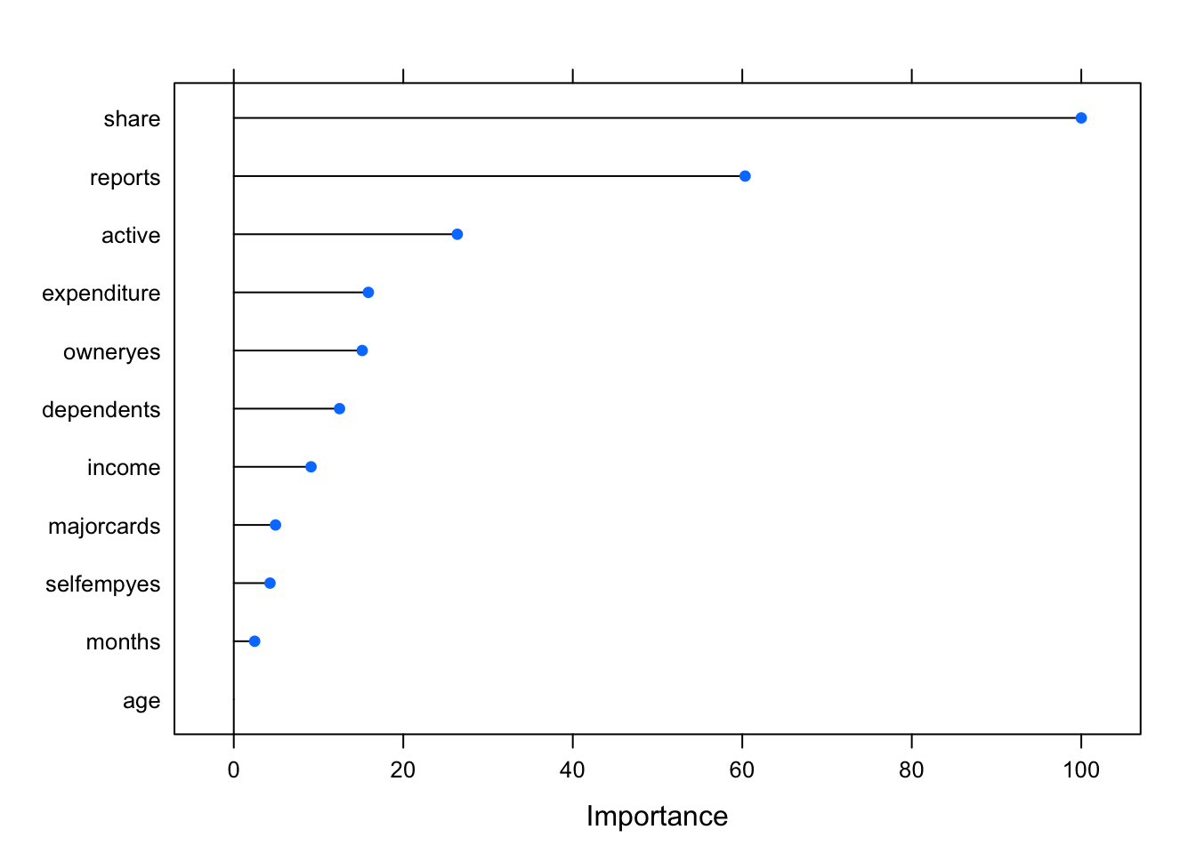
The function automatically scales the importance scores to be between 0 and 100. Using scale = FALSE this normalization step can be avoided.
Unfortunately, since logistic regression has no tuning parameters we can not take advantage of the caret’s feature selection facility (see Variable Selection Using The caret Package).
We will simple retrain the model removing age from the list of predictors. To ensure that each training gets the same data partitions and repeats we need to use the same seed number.
set.seed(123)
credit_glm_mod_1 = train(
  form = card ~ . - age,
  data = train_data,
  trControl = trainControl(method = "cv", number = 5),
  method = "glm",
  family = "binomial"
)

credit_glm_mod_1
## Generalized Linear Model
##
## 990 samples
## 11 predictor
## 2 classes: 'no', 'yes'
##
## No pre-processing
## Resampling: Cross-Validated (5 fold)
## Summary of sample sizes: 792, 792, 791, 793, 792
## Resampling results:
##
## Accuracy Kappa
## 0.885766 0.731973summary(credit_glm_mod_1)##
## Call:
## NULL
##
## Deviance Residuals:
## Min 1Q Median 3Q Max
## -8.49 0.00 0.00 0.00 8.49
##
## Coefficients:
## Estimate Std. Error z value Pr(>|z|)
## (Intercept) -1.018e+15 7.384e+06 -137927087 <2e-16 ***
## reports -4.456e+14 1.611e+06 -276618901 <2e-16 ***
## income 6.523e+13 1.678e+06 38887709 <2e-16 ***
## share 2.292e+16 4.973e+07 460874740 <2e-16 ***
## expenditure -1.527e+12 1.713e+04 -89123688 <2e-16 ***
## owneryes 3.139e+14 4.966e+06 63203076 <2e-16 ***
## selfempyes -3.688e+14 8.173e+06 -45120166 <2e-16 ***
## dependents -9.319e+13 1.861e+06 -50084127 <2e-16 ***
## months -2.331e+11 3.406e+04 -6845424 <2e-16 ***
## majorcards 2.174e+14 5.588e+06 38899415 <2e-16 ***
## active 4.784e+13 3.637e+05 131530123 <2e-16 ***
## ---
## Signif. codes: 0 '***' 0.001 '**' 0.01 '*' 0.05 '.' 0.1 ' ' 1
##
## (Dispersion parameter for binomial family taken to be 1)
##
## Null deviance: 1053.8 on 989 degrees of freedom
## Residual deviance: 9803.9 on 979 degrees of freedom
## AIC: 9825.9
##
## Number of Fisher Scoring iterations: 25Examining the output we can see that the accuracy has increased.
glm_Imp_1 <- varImp(credit_glm_mod_1)
plot(glm_Imp_1)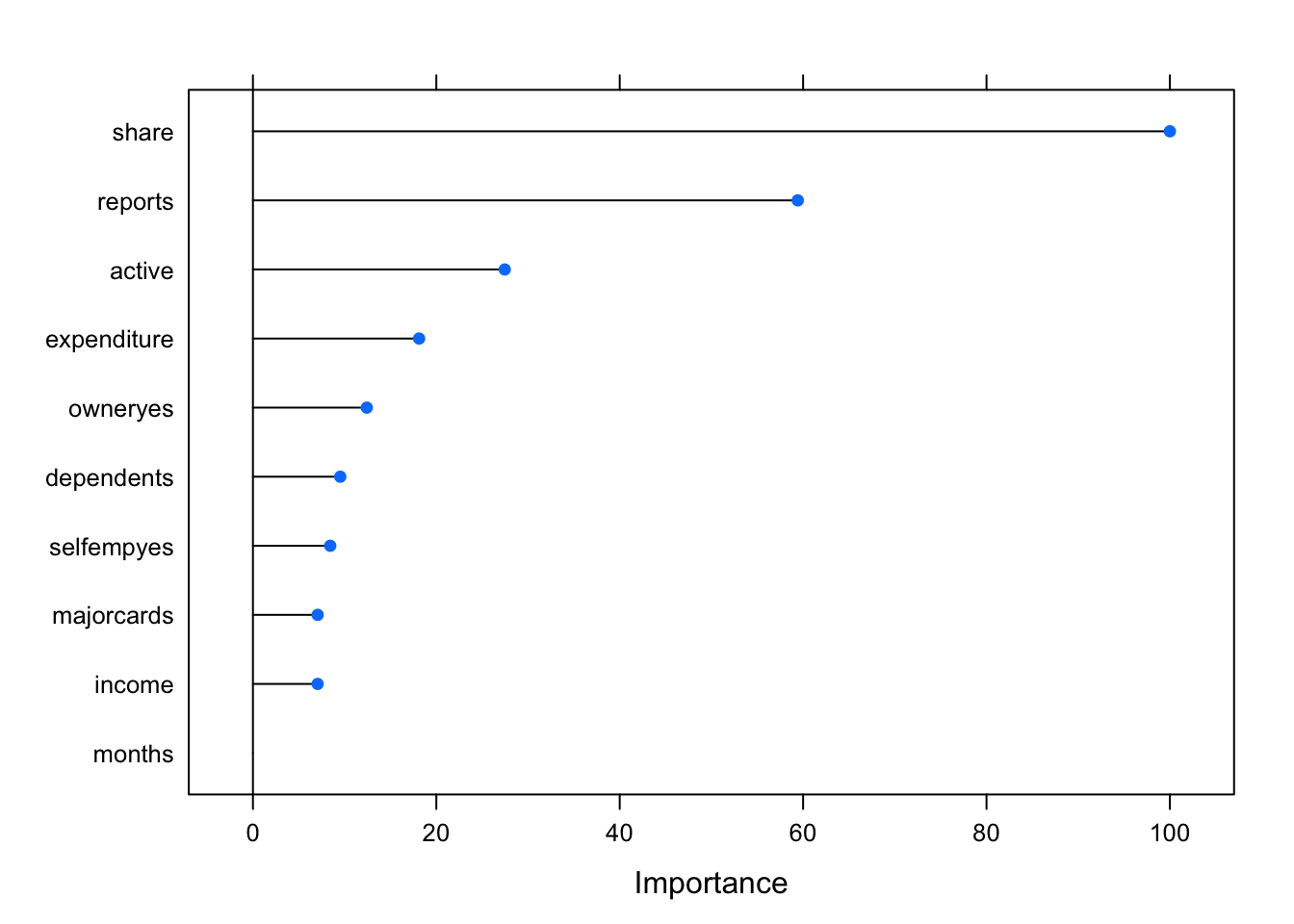
The plot above indicates that predictor months has the lowest impact on the overall model performance.
To compare accuracy between the models we can resample the results of the trained models and compare their accuracy distributions using caret’s resample function and visualise them with the dplot() function. Although logistic regression has no tuning parameters, resampling can still be used to characterise the performance of the model.
set.seed(123) # same resampling specification is used and, since the same random number seed is set
credit_glm_mod$results
## parameter Accuracy Kappa AccuracySD KappaSD
## 1 none 0.8767493 0.6583304 0.06647345 0.1677757credit_glm_mod_1$results## parameter Accuracy Kappa AccuracySD KappaSD
## 1 none 0.885766 0.731973 0.08711903 0.1818121results <- resamples(list(M0 = credit_glm_mod, M1 = credit_glm_mod_1))
summary(results)##
## Call:
## summary.resamples(object = results)
##
## Models: M0, M1
## Number of resamples: 5
##
## Accuracy
## Min. 1st Qu. Median Mean 3rd Qu. Max. NA's
## M0 0.8121827 0.8341709 0.8743719 0.8767493 0.8781726 0.9848485 0
## M1 0.7676768 0.8383838 0.8832487 0.8857660 0.9646465 0.9748744 0
##
## Kappa
## Min. 1st Qu. Median Mean 3rd Qu. Max. NA's
## M0 0.5617898 0.5781585 0.5809996 0.6583304 0.6141825 0.9565217 0
## M1 0.5082604 0.6190476 0.6999139 0.7319730 0.9017161 0.9309268 0dotplot(results)
However, if a strong claim needs to be made about which model is better, we could use statistical hypothesis tests to statistically check if the differences in the results are significant.
modelDifferences <- diff(results)
summary(modelDifferences)
##
## Call:
## summary.diff.resamples(object = modelDifferences)
##
## p-value adjustment: bonferroni
## Upper diagonal: estimates of the difference
## Lower diagonal: p-value for H0: difference = 0
##
## Accuracy
## M0 M1
## M0 -0.009017
## M1 0.8479
##
## Kappa
## M0 M1
## M0 -0.07364
## M1 0.3436The \(p\)-values for the model comparisons are large (0.85 for accuracy and 0.34 for Kappa) indicating that the models fail to show any difference in performance.
YOUR TURN 👇
Practise by doing the following set of exercises:
- Try out data classification using the KNN algorithm using Air Quality Data
AppliedPredictiveModeling::data(twoClassData)
YOUR TURN 👇
Practise by doing the following exercises:
Access the stroke data set from https://tanjakec.github.io/mydata/stroke.csv. Data dictionary of this data set is given in https://tanjakec.github.io/mydata/Stroke_DataDictionary.docx word document.
Split the data into a training and a test set, pre-process the data, and train a model a model of your choice from this section
Predict the response for the test set. What is the value of the performance metric?
Which predictors are most important in the model you have trained?
Train the model using a different method from the previous selection. Don’t forget to initialise the same random number seed as the one used for the previous model training.
Compare the accuracy between the trained models. Which one does it perform better?
Further reading:
“Applied Predictive Modeling” by Max Kuhn
Useful links:
Check Logistic Regression | R Data Analysis Example which uses categorical predictors.
Binary Response and Logistic Regression Analysis
Predictive Modeling with R and the caret Package, useR! 2013, by Max Kuhn
caret package webinar by Max Khun
Intro to Machine Learning with R & caret
Data to practise:
http://archive.ics.uci.edu/ml/index.php
Machine Learning on Bankruptcy
© 2020 Tatjana Kecojevic